Implementation of an incompressible Navier-Stokes model
Objective of this 4th tutorial
The objective is to start from a kernel which simulates an Advection-Diffusion Equation and modify it to simulate a Navier-Stokes model for single-phase applications. The verifications will be done with the classic test case of “lid driven cavity flow”.
1. Create a new kernel NS
Create a new kernel NS
You can refer to Tuto 1 & 2 where all commands have been presented in detail:
Copy the kernel
ADE_for_NSand rename itNavier-Stokes_Tutorialin directoryLBM_Saclay_Rech-Dev/src/kernels/Go to your new folder
Navier-Stokes_Tutorialand replace all files with extension_ADEby_NSEdit your files and replace
_ADEwith_NSIn file
Setup.hreplace the problem nameADEbyNSCreate your
Makefilewith option-DPROBLEM=Navier-Stokes_Tutorialand compile
2. Modifications inside each file of NS
enum ComponentIndex
In
enum ComponentIndex, add a new indexIDfor density \(\rho\)
Solution
enum ComponentIndex {
  IU     , /*!< X velocity / momentum index */
  IV     , /*!< Y velocity / momentum index */
  IW     , /*!< Z velocity / momentum index */
  IC     , /*!< Phase field index */
  ID     ,
  COMPONENT_SIZE /*!< invalid index, just counting number of fields */
};
struct index2names
In
struct index2names, add a new stringrhoto write the density \(\rho\) in the output file
Solution
// insert some fields
map[IC ] = "comp";
map[IU ] = "vx";
map[IV ] = "vy";
map[IW ] = "vz";
map[ID ] = "rho";
return map;
Read and declare Navier-Stokes parameters in ModelParams
The Navier-Stokes equations involve two main input parameters: the kinematic viscosity \(\nu\) and the initial density \(\rho\). A new flag flow is also introduced to simulate or not the Navier-Stokes model. If flow=0.0 then the ADE is simulated, else if flow=1.0 then the NS model is simulated.
Read and declare the Navier-Stokes parameters in
ModelParams
Solution
Read parameters in input file:
flow     = configMap.getFloat("params", "flow"    , 0.0);
nu       = configMap.getFloat("params", "nu"      , 1.0);

rho_init = configMap.getFloat("init"  , "rho_init", 1.0);
Declare them as
real_tat the end ofModelParams
Solution
real_t flow, nu, rho_init;
Add specific functions for Navier-Stokes
Add a new function
tau_NSfor relaxation rate \(\tau_{NS}\)
Solution
tau_NS// ======================================================= // relaxation rate for kinematic viscosity KOKKOS_INLINE_FUNCTION real_t tau_NS(EquationTag1 tag, const LBMState &lbmState) const { real_t tau = 0.5 + (e2 * nu * dt / SQR(dx)); return (tau); }
Function setup_collider with BGK
The function setup_collider is adapted for ADE. It must be compteled to simulate Navier-Stokes equations.
Add a new block
if-else iffor flagflow=0.0andflow=1.0and move the ADEsetup_colliderinside the first condition.
Solution
LBMState lbmState;
Base::template setupLBMState2<LBMState, COMPONENT_SIZE>(IJK, lbmState);

if (Model.flow == 0.0) {
  const real_t M0     = Model.MomentM0(tag, lbmState);
  const RVect<dim> uc = Model.MomentM1<dim>(tag, lbmState);
  const real_t M2     = Model.MomentM2(tag, lbmState);

  // compute collision rate
  collider.tau = Model.tau(tag, lbmState);

  // ipop = 0
  collider.f[0]   = Base::get_f_val(tag, IJK, 0);
  collider.S0[0]  = 0.0 ;
  collider.feq[0] = w[0]*M0;

  // ipop > 0
  for (int ipop = 1; ipop < npop; ++ipop) {
     collider.f[ipop]   = this->get_f_val(tag, IJK, ipop);
     collider.S0[ipop]  = 0.0 ;
     collider.feq[ipop] = w[ipop] * (M2 + c_cs2 * Base::compute_scal(ipop, uc));
  }
}

else if (Model.flow == 1.0) {
}
Complete the
else ifpart with the NSsetup_collider
Solution
else if (Model.flow == 1.0) {
  FState GAMMA;
  const real_t rho = lbmState[ID] ;
  collider.tau     = Model.tau_NS(tag, lbmState);
  real_t scalUU    = SQR(lbmState[IU]) + SQR(lbmState[IV]);
  for (int ipop    = 0; ipop < npop; ++ipop) {
     real_t scalUC = c * Base::compute_scal(ipop, lbmState[IU], lbmState[IV]);
     GAMMA[ipop]   = e2*scalUC/c2 + 0.5*SQR(e2*scalUC)/SQR(c2) - 0.5*e2*scalUU/c2;
     collider.feq[ipop] = rho * w[ipop] * (1.0 +  GAMMA[ipop]);
     collider.f[ipop]   = Base::get_f_val(tag, IJK, ipop);
     collider.S0[ipop]  = 0.0 ;
  }
}
Function make_boundary with BGK
The function make_boundary is adapted for ADE. It must be compteled for Navier-Stokes boundary conditions.
Add a new block
if-else iffor flagflow=0.0andflow=1.0and move the ADEsetup_colliderinside the first condition.
Solution
const real_t c = dx / dt;
const real_t c_cs2 = Model.e2 / (c * Model.rho_init);

// ADE boundary
if (Model.flow == 0.0) {
  if (Base::params.boundary_types[BOUNDARY_EQUATION_1][faceId] == BC_ANTI_BOUNCE_BACK) {
     real_t boundary_value = Base::params.boundary_values[BOUNDARY_PHASE_FIELD][faceId];
     for (int ipop = 0; ipop < npop; ++ipop)
        this->compute_boundary_antibounceback(tagC, faceId, IJK, ipop, boundary_value);
  }

  else if (Base::params.boundary_types[BOUNDARY_EQUATION_1][faceId] == BC_ZERO_FLUX) {
     for (int ipop = 0; ipop < npop; ++ipop)
        this->compute_boundary_bounceback(tagC, faceId, IJK, ipop, 0.0);
  }
}
// NS boundary
else if (Model.flow == 1.0) {
}
Complete the
else ifpart with three boundary conditions for Navier-Stokes (pressure, no-slip and velocity)
Solution
else if (Model.flow == 1.0) {
  // Pressure imposed
  if (Base::params.boundary_types[BOUNDARY_EQUATION_1][faceId] == BC_ANTI_BOUNCE_BACK) {
     real_t boundary_value = this->params.boundary_values[BOUNDARY_PRESSURE][faceId];
     for (int ipop = 0; ipop < npop; ++ipop) {
        this->compute_boundary_antibounceback(tagC, faceId, IJK, ipop, boundary_value);
     }
  }
  // No-slip boundary condition
  else if (Base::params.boundary_types[BOUNDARY_EQUATION_1][faceId] == BC_ZERO_FLUX) {
     for (int ipop = 0; ipop < npop; ++ipop)
        this->compute_boundary_bounceback(tagC, faceId, IJK, ipop, 0.0);
  }
  // Velocity imposed (e.g. for test case of lid driven cavity flow)
  else if (Base::params.boundary_types[BOUNDARY_EQUATION_1][faceId] == BC_BOUNCEBACK) {
     real_t boundary_vx = this->params.boundary_values[BOUNDARY_VELOCITY_X][faceId];
     real_t boundary_vy = this->params.boundary_values[BOUNDARY_VELOCITY_Y][faceId];
     real_t value;
     for (int ipop = 0; ipop < npop; ++ipop) {
        value = c_cs2 * this->compute_scal_Ebar(ipop, boundary_vx, boundary_vy);
        this->compute_boundary_bounceback(tagC, faceId, IJK, ipop, value);
     }
  }
}
Function init_macro with BGK
The function init_macro is adapted for ADE. It must be compteled for Navier-Stokes initial condition.
Add a new block
if-else iffor flagflow=0.0andflow=1.0and move the ADE initialization inside the first condition.
Solution
real_t x, y;
this->get_coordinates(IJK, x, y);

if (Model.flow == 0.0) {
  real_t c    = 0.0;
  real_t xphi = 0.0;
  real_t vx   = 0.0;
  real_t vy   = 0.0;

  if (Model.initType == ADE_GAUSSIAN) {
     c  = Model.ampl * exp( - ( SQR(x-Model.x0) / (2 * SQR(Model.sigmax)) +
           SQR(y-Model.y0) / (2 * SQR(Model.sigmay)) )) ;
     vx = Model.initVX;
     vy = Model.initVY;
  }

  this->set_lbm_val(IJK, IC, c);
  this->set_lbm_val(IJK, IU, vx);
  this->set_lbm_val(IJK, IV, vy);
}

else if (Model.flow == 1.0) {
}
Complete the
else ifpart withrho_initand null velocity and save in array with appropriate indices
Solution
else if (Model.flow == 1.0) {
  real_t rho = Model.rho_init;
  real_t vx  = Model.initVX  ;
  real_t vy  = Model.initVY  ;

  this->set_lbm_val(IJK, ID, rho);
  this->set_lbm_val(IJK, IU, vx);
  this->set_lbm_val(IJK, IV, vy);
}
Function update_macro with BGK
The function update_macro is adapted for ADE. It must be compteled for Navier-Stokes.
Add a new block
if-else iffor flagflow=0.0andflow=1.0and move the ADE initialization inside the first condition.
Solution
// get local coordinates
real_t x, y;
this->get_coordinates(IJK, x, y);

if (Model.flow == 0.0) {
  // compute moments of distribution equations
  real_t moment_c = 0.0;

  for (int ipop = 0; ipop < npop; ++ipop) {
     moment_c += Base::get_f_val(tagC, IJK, ipop);
  }

  // store old values of macro fields
  LBMState lbmStatePrev;

  // get source terms and compute new macro fields
  const real_t c  = moment_c;
  const real_t vx = Model.initVX;
  const real_t vy = Model.initVY;

  // update macro fields
  this->set_lbm_val(IJK, IC , c );
  this->set_lbm_val(IJK, IU , vx );
  this->set_lbm_val(IJK, IV , vy );
}

else if (Model.flow == 1.0) {
}
Complete the
else ifpart for \(\rho,u_x,u_y\) and save in array with appropriate indices
Solution
else if (Model.flow == 1.0) {
  const real_t dt = Model.dt;
  const real_t dx = Model.dx;
  const real_t c  = dx/dt ;
  // compute moments of distribution equations
  real_t moment_rho = 0.0;
  real_t moment_VX  = 0.0;
  real_t moment_VY  = 0.0;
  for (int ipop = 0; ipop < npop; ++ipop) {
     moment_rho += Base::get_f_val(tagC, IJK, ipop);
     moment_VX  += Base::get_f_val(tagC, IJK, ipop) * E[ipop][IX] * c ;
     moment_VY  += Base::get_f_val(tagC, IJK, ipop) * E[ipop][IY] * c ;
  }
  // Save with appropriate indices
  const real_t rho = moment_rho;
  const real_t vx  = moment_VX / rho ;
  const real_t vy  = moment_VY / rho ;

  this->set_lbm_val(IJK, ID , rho);
  this->set_lbm_val(IJK, IU , vx );
  this->set_lbm_val(IJK, IV , vy );
}
3. Verification of your implementation
The test case of validation is the “lid driven cavity flow”. The input file is Tuto04_NS_Cavity-flow-Re1000.ini in the directory run_training_lbm/Tutorial04_Navier-Stokes.
Run and post-process your results
Go to the appropriate folder and run LBM_Saclay
$ cd LBM_Saclay_Rech-Dev/run_training_lbm/Tutorial04_Navier-Stokes
$ ../../build_NS/src/LBM_saclay Tuto04_NS_Cavity-flow-Re1000.ini
Once the computation is complete, extract from your final
.vtifile one profile \(u_x\) as a function of \(y\) with paraview 5.12
$ path_to_pvpython/pvpython Extract-Profile_Ux-y_Re1000.pvpyThe output is a
.csvfile calledProfile_LBM_Cavity_BGK_1000_Ux.csv.
Compare with the analytical solution written in the python script
Compare_Ghia_Profile_Ux-y_Re1000.py
$ python Compare_Ghia_Profile_Ux-y_Re1000.pyYou must obtain Fig Fig. 48
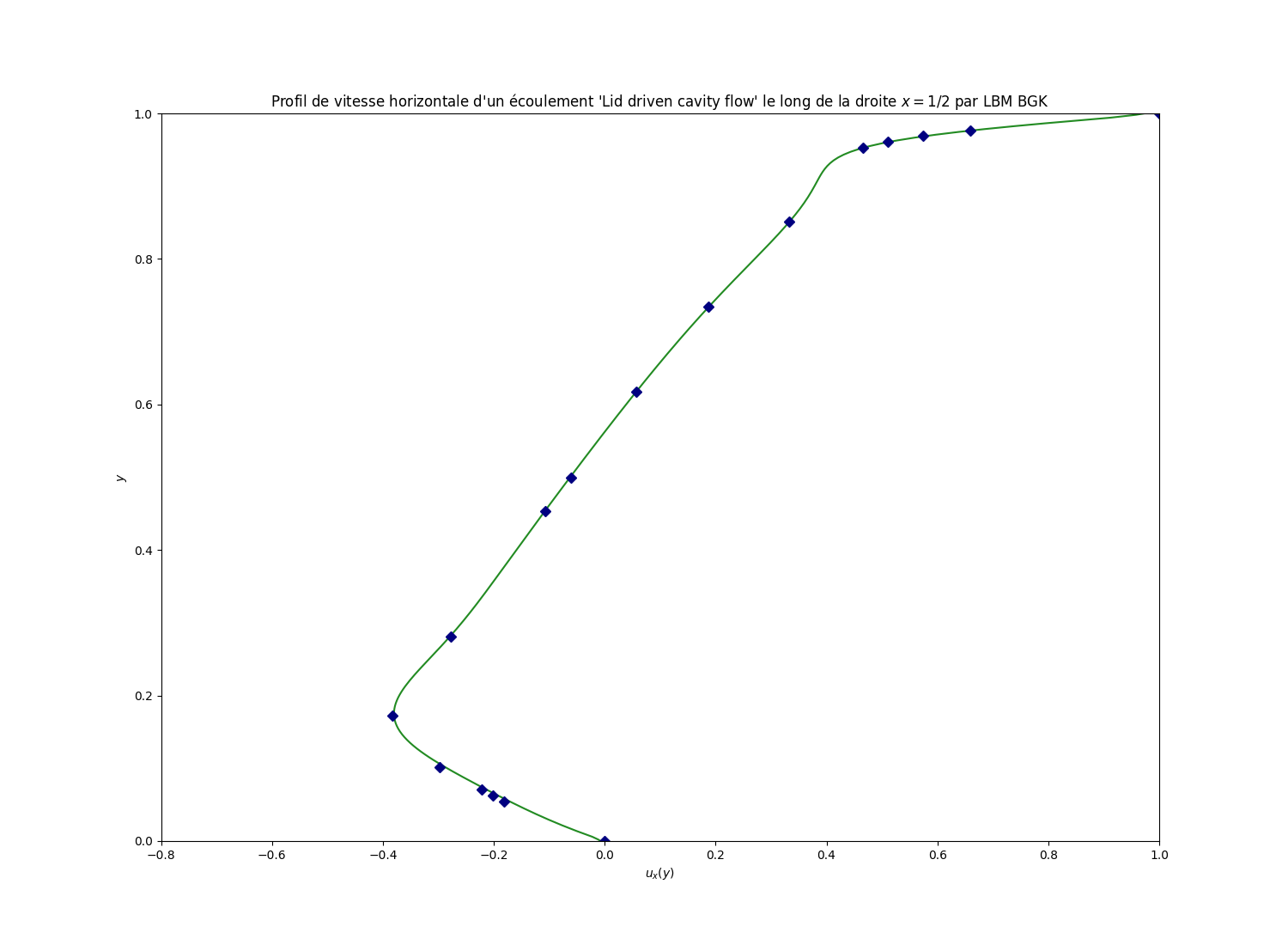
Fig. 48 Comparison between LBM and Ghia et al. reference solution
Section author: Alain Cartalade