Implementation of a crystal growth model

Objective of this 3rd tutorial

The starting point is the kernel ACT of the second tutorial. That kernel will be modified here in order to simulate the growth of one crystal.

Mathematical model

The mathematical model is composed of one dimensionless temperature equation which writes:

(260)\[\frac{\partial\theta}{\partial t}=D\boldsymbol{\nabla}^{2}\theta+\frac{1}{2}\frac{\partial\psi}{\partial t}\]

The phase-field equation is slightly more complex than the previous one in the 2nd tutorial:

(261)\[\tau_{0}{\color{red}a_{s}^{2}(\boldsymbol{n})}\frac{\partial\psi}{\partial t}=W_{0}^{2}\boldsymbol{\nabla}\cdot\left[{\color{red}a_{s}^{2}(\boldsymbol{n})}\boldsymbol{\nabla}\psi\right]+\boldsymbol{\nabla}\cdot{\color{blue}\boldsymbol{\mathcal{N}}(\boldsymbol{n})}+(1-\psi^{2})\left[\psi-\lambda\theta(1-\psi^{2})\right]\]

where the anisotropy function writes:

(262)\[{\color{red}a_{s}(\boldsymbol{n})}=1-3\epsilon_{s}+4\epsilon_{s}\sum_{\alpha=x,y,z}n_{\alpha}^{4}\]

and the vector $\boldsymbol{\mathcal{N}}$ by

(263)\[{\color{blue}\boldsymbol{\mathcal{N}}(\boldsymbol{n})}=W_{0}^{2}\bigl|\boldsymbol{\nabla}\psi\bigr|^{2}{\color{red}a_{s}(\boldsymbol{n})}\frac{\partial{\color{red}a_{s}(\boldsymbol{n})}}{\partial(\partial_{\alpha}\psi)}\]

Objective

Until now, only the standard BGK collider was used in our implementation. In this tutorial, we will see how to

use another LBM_Saclay collider, based on BGK (but modified) to take into account the $\tau_{0}{\color{red}a_{s}^{2}(\boldsymbol{n})}$ in front of the partial derivative $\partial \psi/\partial t$.
modify the setup_collider for $\boldsymbol{\nabla}\cdot{\color{blue}\boldsymbol{\mathcal{N}}(\boldsymbol{n})}$

1. Use a new collision operator for the phase-field equation in your kernel

Several collision operators are already implemented in Collision_operators.h. The most popular are BGK, TRT and MRT. Here we will use a BGK operator, slightly modified and involving a non-local term. It is mainly used to take into account a time-evolving factor in front the partial derivative in time. In LBM_Saclay, that operator is called BGKColliderTimeFactor.

File Problem_ACT.h

Function update_f()

For BGK the update is currently

if (params.collisionType2 == BGK) {
  update1eq<EquationTag2, BGKCollider<dim, npop>>();

Modify it for BGKColliderTimeFactor

File LBMScheme_ACT.h

struct LBMScheme

Currently only two collisions are defined

using BGK_Collider = BGKCollider<dim, npop>;
using MRT_Collider = MRTCollider<dim, npop>;

Define a new collision

Add a new empty function setup_collider for EquationTag2 with BGK_Collider_Time_Factor

2. Modifications inside each file for implementing a crystal growth model

File Index_ACT.h

Declaration of new fields

From the previous tutorialn, in enum ComponentIndex, the indices for macroscopic fields are:

enum ComponentIndex {
  IU     , /*!< X velocity / momentum index */
  IV     , /*!< Y velocity / momentum index */
  IW     , /*!< Z velocity / momentum index */
  ITEMP  , /*!< Temperature index */
  IPHI   , /*!< Phase field index */
  IDPHIDT,
  COMPONENT_SIZE /*!< invalid index, just counting number of fields */
};

Add for components of gradient of $\phi$

File Models_ACT.h

Read and declare all parameters in ModelParams

The Allen-Cahn equation involves three parameters: the interface thickness $W$ and the mobility $M_\phi$ and the interface temperature $\theta_I$.

Read and declare Allen-Cahn parameters in ModelParams

Add condition for initial condition

Currently only one condition exits for intial condition:

if (initTypeStr == "gaussian") initType = ADE_GAUSSIAN;
else if (initTypeStr == "vertical") initType = PHASE_FIELD_INIT_VERTICAL;

Add the necessary condition for one initialization

Add specific functions for temperature equation

Modify function Source_TEMP with factor 1/2 (be careful with the positive sign)

Add specific functions of crystal growth functions in the phase-field equation

Add another source term

Add a new function tau_PHI_Crystal for collision rate using the anaisotropy function $a_s()\boldsymbol{n}$

Add a new hyperbolic tangent function phi1 for initial condition

Add a new function compute_anisotropy for computing the anisotropy function $a_s(\boldsymbol{n})$

Add a new function compute_anisotropy_vector

File LBMScheme_ACT.h

Write a new function setup_collider with BGK_Collider_Time_Factor

Fill the new setup_collider for phase-field equation

Function init_macro

After the initialization for ADE_GAUSSIAN:

if (Model.initType == ADE_GAUSSIAN) {
  c  = Model.ampl * exp( - ( SQR(x-Model.x0) / (2 * SQR(Model.sigmax)) + SQR(y-Model.y0) / (2 * SQR(Model.sigmay)) )) ;
  vx = Model.initVX;
  vy = Model.initVY;
}
else if (Model.initType == PHASE_FIELD_INIT_VERTICAL) {
  xphi = x - Model.x0;
  c    = Model.undercooling ;
}

real_t phi = Model.phi0(xphi);

Write an initial condition corresponding to keywords PHASE_FIELD_INIT_SPHERE

Save in appropriate arrays

Function update_macro_grad

That function is currently empty

KOKKOS_INLINE_FUNCTION
void update_macro_grad(IVect<dim> IJK) const
{
}

Add the computation of gradient

File InitConditionsTypes.h

Add the keywords of initial conditions

In file InitConditionsTypes.h, two keywords are currently declared:

enum InitCondition{
   PHASE_FIELD_INIT_UNDEFINED,
   ADE_GAUSSIAN,
   PHASE_FIELD_INIT_VERTICAL
};

Simply add after PHASE_FIELD_INIT_VERTICAL the new keyword for Allen-Cahn: PHASE_FIELD_INIT_SPHERE.

3. Verifications of your implementation

Run and post-process your results

An input file Crystal-Equiaxe.ini is given in the folder Tutorial03_Crystal-Growth.

Run LBM_Saclay with that input file
Post-process your .vti outputs with the pvpython input file Video-plus-Contour.pvpy for paraview 5.11

$ /tmp_formation/LBM_Saclay/ParaView/ParaView-5.11.0-MPI-Linux-Python3.9-x86_64/bin/pvpython Video-plus-Contour.pvpy
The outputs are several .csv files plus one video (.avi format).

Run the video generated by the post-processing

$ vlc Vid-Crystal-Growth_Equiaxe.avi

Video: simulation of 2D crystal growth

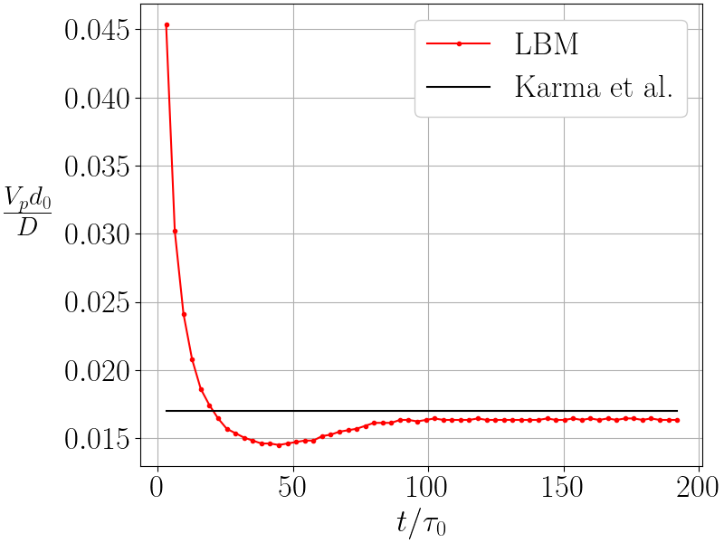
Compare the evolution of velocity tip with the steady reference.

$ python tip_velocity_contour.py
You must obtain Fig. Fig. 47

Fig. 47 Comparison between LBM and reference solution of Karma-Rappel

Section author: Alain Cartalade & Capucine Méjanès

Implementation of a crystal growth model

Objective of this 3rd tutorial

1. Use a new collision operator for the phase-field equation in your kernel

2. Modifications inside each file for implementing a crystal growth model

3. Verifications of your implementation

Table of Contents

Previous topic

Next topic