Implementation of a Navier-Stokes/Cahn-Hilliard model

Objective of this 5th tutorial

The objective is to implement in LBM_Saclay, the Navier-Stokes/Cahn-Hilliard model. The starting point is the kernel CH implemented in the first tutorial. It will be extended here with the Navier-Stokes (NS) equations and renamed NSCH.

Mathematical model & LBM scheme

The model summarized in Summary of Navier-Stokes/phase-field model composed of incompressible Navier-Stokes equations Eqs. (503) - (507) coupled with a Cahn-Hilliard equation Eq. (508). Two forces appear in that model: 1) the capillary force defined by Eq. (500) $\boldsymbol{F}_c=\mu_{\phi}\boldsymbol{\nabla}\phi$ and 2) the gravity force defined by $\boldsymbol{F}_g=\varrho\boldsymbol{g}$.
The equilibrium distribution function for incompressible Navier-Stokes is the version 2 presented in LBM scheme for incompressble NS. The scheme works on a dimensionless pressure $p^{\star}_h$. It needs to add a viscous force $\boldsymbol{F}_v$ (Eq. (210)) and a pressure force $\boldsymbol{F}_p$ (Eq. (209)) to be consistent with the continuous model.
Expression of viscous force in LBM

LBM formulation of $\boldsymbol{F}_v$

(264)\[\boldsymbol{F}_{v}=-\frac{\nu}{c_{s}^{2}\delta t}\sum_{i}\boldsymbol{c}_{i}(\boldsymbol{c}_{i}\cdot\boldsymbol{\nabla}\varrho)f_{i}^{\star}\]

where

(265)\[f_{i}^{\star}=(\boldsymbol{M}^{-1}\boldsymbol{S}\boldsymbol{M}(\boldsymbol{f}-\boldsymbol{f}^{eq}))_{i}\]

For each component

\[\begin{split}F_{v,x}=-\frac{\nu}{c_{s}^{2}\delta t}\sum_{i=0}^{N_{pop}}c_{ix}\left[c_{ix}(\partial_{x}\varrho)+c_{iy}(\partial_{y}\varrho)+c_{iz}(\partial_{z}\varrho)\right]f_{i}^{\star}\\ F_{v,y}=-\frac{\nu}{c_{s}^{2}\delta t}\sum_{i=0}^{N_{pop}}c_{iy}\left[c_{ix}(\partial_{x}\varrho)+c_{iy}(\partial_{y}\varrho)+c_{iz}(\partial_{z}\varrho)\right]f_{i}^{\star}\\ F_{v,z}=-\frac{\nu}{c_{s}^{2}\delta t}\sum_{i=0}^{N_{pop}}c_{iz}\left[c_{ix}(\partial_{x}\varrho)+c_{iy}(\partial_{y}\varrho)+c_{iz}(\partial_{z}\varrho)\right]f_{i}^{\star}\end{split}\]

Objective

In this tutorial, we will see how to

add a new equation (like tuto 2)
add a setup_collider function relative to NS equations
add external force terms $\boldsymbol{F}_c$ and $\boldsymbol{F}_g$
add force terms $\boldsymbol{F}_v$ and $\boldsymbol{F}_p$ for consistency

1. Create a new kernel `NSCH`

Create a new kernel NSCH

You can refer to Tuto 1 & 2 where all commands have been presented in detail:

Copy your kernel CH and rename it NSCH_Tutorial in directory LBM_Saclay_Rech-Dev/src/kernels/
Go to your new folder NSCH_Tutorial and replace all files with extension _CH by _NSCH
Edit your files and replace _CH with _NSCH
In file Setup.h replace the problem name CH by NSCH
Create your Makefile with option -DPROBLEM=NSCH_Tutorial and compile

2. Add a new equation in your kernel `NSCH`

The mathematical model is currently composed of one Cahn-Hilliard equation. It is necessary to add one supplementary equation.

File Problem_ACT.h

Problem

The number of equation is currently 1

Base::nbEqs = 1;

const int isize = params.isize;
const int jsize = params.jsize;
const int ksize = params.ksize;

Modify it for two equations

Function init_f()

The initialization is currently performed only for one equation:

if (params.collisionType1 == BGK) {
     init1eq<EquationTag1, BGKCollider<dim, npop>>();
} else if (params.collisionType1 == MRT) {
     init1eq<EquationTag1, MRTCollider<dim, npop>>();
}

Add a new block if - else if for EquationTag2

Function update_f()

The update is also performed only for one equation:

if (params.collisionType1 == BGK) {
  update1eq<EquationTag1, BGKCollider<dim, npop>>();
} else if (params.collisionType1 == MRT) {
  update1eq<EquationTag1, MRTCollider<dim, npop>>();
}

Add a new block if - else if for EquationTag2

Function make_boundaries()

The update of bounday conditions is also performed for a single equation

this->bcPerMgr.make_boundaries(scheme.f1, BOUNDARY_EQUATION_1);

Add a new line for f2 and BOUNDARY_EQUATION_2

File LBMScheme_ACT.h

Function struct LBMScheme

Add a new tag tagNS for EquationTag2

Add two empty functions called setup_collider for EquationTag2 with respectively BGK and MRT collisions

Function make_boundary

The boundary conditions are applied only for Cahn-Hilliard equation

// phi boundary
if (Base::params.boundary_types[BOUNDARY_EQUATION_1][faceId] == BC_ANTI_BOUNCE_BACK) {
  real_t boundary_value = Base::params.boundary_values[BOUNDARY_CONCENTRATION][faceId];

  for (int ipop = 0; ipop < npop; ++ipop)
     this->compute_boundary_antibounceback(tagC, faceId, IJK, ipop, boundary_value);
}
else if (Base::params.boundary_types[BOUNDARY_EQUATION_1][faceId] == BC_ZERO_FLUX) {
  for (int ipop = 0; ipop < npop; ++ipop)
     this->compute_boundary_bounceback(tagNS, faceId, IJK, ipop, 0.0);
}

Add a new block if - else if for BOUNDARY_EQUATION_2 and tagNS with keyword BOUNDARY_PRESSURE

3. Modifications inside each file of `NSCH`

File Index_NSCH.h

Declaration of new fields

In enum ComponentIndex, only the indices relative to Cahn-Hilliard model are declared:

enum ComponentIndex {
  IU     , /*!< X velocity / momentum index */
  IV     , /*!< Y velocity / momentum index */
  IW     , /*!< Z velocity / momentum index */
  IC     , /*!< Phase field index */
  IMU    , /*!< Chemical potential */
  ILAPLAC,     /*!< Laplacien of Phase field */
  COMPONENT_SIZE /*!< invalid index, just counting number of fields */
};

Complete the list with hydrodynamics indices density $\varrho$, hydrodynamic pressure $p_h$, gradient $\boldsymbol{\nabla}\phi$, gradient $\boldsymbol{\nabla}\varrho$ and total force $\boldsymbol{F}_{tot}$.

Add new outputs

In struct index2names only the strings for Cahn-Hilliard model are written:

map[IC ] = "comp";
map[IU ] = "vx";
map[IV ] = "vy";
map[IW ] = "vz";
map[IMU] = "mu";

Add a new outputs for density and pressure (and more if wanted).

File Models_NSCH.h

Read and declare Navier-Stokes parameters in ModelParams

The Navier-Stokes equations involve several parameters: the kinematic viscosity $\nu_1$ of fluid 1 (respectively $\nu_2$ of fluid 2), the density $\rho_1$ ($\rho_2$). The surface tension $\sigma$ has already been read as input paramater for Cahn-Hilliard equation. Also read the components of gravity $\boldsymbol{g}=(g_x,g_y,g_z)$ (gx, gy, gz)

Read and declare the Navier-Stokes parameters in ModelParams

Declare them as real_t at the end of ModelParams

From Tuto 1, three initial conditions are currently implemented

if (initTypeStr == "random") initType = RANDOM_SPINODAL;
else if (initTypeStr == "nucleation") initType = RANDOM_NUCLEATION;
else if (initTypeStr == "serpentine") initType = SERPENTINE;

Add a new else if condition for vertical (see Tuto 2)

Add specific functions for Navier-Stokes

Add a new harmonic function tau_NS for relaxation rate $\tau_{NS}$

Add a new function interpol_rho for linear interpolation of density $\varrho=\rho_1\phi+\rho_2(1-\phi)$

Add a new function force_P for pressure force $\boldsymbol{F}_p=-p_h/\varrho(\phi)\boldsymbol{\nabla}\varrho$

Add a new function force_G for gravity force $\boldsymbol{F}_g=\varrho\boldsymbol{g}$

Add a new function force_TS for surface tension force $\mu_{\phi}\boldsymbol{\nabla}\phi$

File LBMScheme_NSCH.h

Function setup_collider with BGK

From stage 2, the function setup_collider with BGK_Collider is currently empty. It must be filled to simulate Navier-Stokes equations.

Solution

KOKKOS_INLINE_FUNCTION
void setup_collider(EquationTag2 tag, const IVect<dim> &IJK, BGK_Collider &collider) const
{
  // Paramètres pour la simulation
  const real_t dx = Model.dx;
  const real_t dt = Model.dt;
  const real_t c = dx / dt;
  const real_t cs2 = SQR(c) / Model.e2;
  // Stockage des anciennes grandeurs macroscopiques
  LBMState lbmState;
  Base::template setupLBMState2<LBMState, COMPONENT_SIZE>(IJK, lbmState);

  // Calcul du tau de collision
  collider.tau = Model.tau_NS(lbmState);

Equilibrium distribution function Eq. (202) without variable change

  // Equilibrium without force term
  FState GAMMA;
  if (dim == 2) {
     real_t scalUU    = SQR(lbmState[IU]) + SQR(lbmState[IV]);
     for (int ipop    = 0; ipop < npop; ++ipop) {
        real_t scalUC = c * Base::compute_scal(ipop, lbmState[IU], lbmState[IV]);
        GAMMA[ipop]   = scalUC / cs2 + 0.5 * SQR(scalUC) / SQR(cs2) - 0.5 * scalUU / cs2;
        real_t feqbar = w[ipop] * (lbmState[IP] / (cs2 * lbmState[ID]) + GAMMA[ipop]);
        collider.feq[ipop] = feqbar;
        collider.f[ipop]   = Base::get_f_val(tag, IJK, ipop);
     }

Computation of force terms $\boldsymbol{F}_c$, $\boldsymbol{F}_g$ and $\boldsymbol{F}_p$ defined in file Models_NSCH.h

     // Computation of force terms defined in models
     RVect<dim> ForceTS = Model.force_TS<dim>(lbmState);
     RVect<dim> ForceG  = Model.force_G<dim>(lbmState);
     RVect<dim> ForceP  = Model.force_P<dim>(lbmState);

Computation of viscous force $F_{v,x}$ and $F_{v,y}$ Eq. (264) & Eq. (265). For BGK collision only one relaxation rate is involved. It appears in factor coeffV.

     // Computation of viscous force
     RVect<dim> ForceV;
     const real_t nu = Model.nu0 * Model.nu1 / (((1.0 - lbmState[IPHI]) * Model.nu1) + ((lbmState[IPHI]) * Model.nu0));
     real_t coeffV = - nu / (cs2 * dt * collider.tau);
     ForceV[IX] = 0.0;
     ForceV[IY] = 0.0;
     for (int alpha = 0; alpha < npop; ++alpha) {
        ForceV[IX] += E[alpha][IX] * E[alpha][IX] * lbmState[IDRHODX] * (collider.f[alpha] - collider.feq[alpha]) +
                      E[alpha][IX] * E[alpha][IY] * lbmState[IDRHODY] * (collider.f[alpha] - collider.feq[alpha]);
        ForceV[IY] += E[alpha][IY] * E[alpha][IX] * lbmState[IDRHODX] * (collider.f[alpha] - collider.feq[alpha]) +
                      E[alpha][IY] * E[alpha][IY] * lbmState[IDRHODY] * (collider.f[alpha] - collider.feq[alpha]);
     }
     ForceV[IX] = coeffV * ForceV[IX];
     ForceV[IY] = coeffV * ForceV[IY];

Computation of total force $\boldsymbol{F}_{tot}$ and save in array with appropriate indices IFX and IFY

     // Calcul et enregistrement du terme source total
     RVect<dim> ForceTot;
     ForceTot[IX] = ForceG[IX] + ForceP[IX] + ForceTS[IX] + ForceV[IX];
     ForceTot[IY] = ForceG[IY] + ForceP[IY] + ForceTS[IY] + ForceV[IY];

     this->set_lbm_val(IJK, IFX, ForceTot[IX]);
     this->set_lbm_val(IJK, IFY, ForceTot[IY]);

Correction of equilibrium (variable change) with total force term ForceTot[IX] & ForceTot[IY]

     // Add force term in equilibrium
     for (int ipop = 0; ipop < npop; ++ipop) {
        collider.S0[ipop]  = dx * w[ipop] / (lbmState[ID] * cs2) * Base::compute_scal(ipop, ForceTot[IX], ForceTot[IY]);
        collider.feq[ipop] = collider.feq[ipop] - 0.5 * (collider.S0[ipop]);
     }
  }
} // end of setup_collider for composition equation

Function init_macro

Write (or copy-paste from tuto 2) an initial condition corresponding to keywords PHASE_FIELD_INIT_VERTICAL

Save in appropriate arrays

Function update_macro

Update necessary fields

Function update_macro_grad

Currently the function contains the laplacian computation for chemical potential.

KOKKOS_INLINE_FUNCTION
void update_macro_grad(IVect<dim> IJK) const {
  real_t laplace_c = Base::compute_laplacian(IJK, IC, BOUNDARY_EQUATION_1);
  Base::set_lbm_val(IJK, ILAPLAC, laplace_c);
}

Add computation of gradients

File InitConditionsTypes.h

Add the keywords of initial conditions

In file InitConditionsTypes.h, two keywords are currently declared:

enum InitCondition{
  PHASE_FIELD_INIT_UNDEFINED,
  ADE_GAUSSIAN,
  RANDOM_SPINODAL,
  RANDOM_NUCLEATION,
  SERPENTINE
};

Add the new keyword for initial condition PHASE_FIELD_INIT_VERTICAL

4. Verification of your implementation

The test case of validation is the double-Poiseuille flow. The input file is Test-Tuto04_Double_Poiseuille_BGK.ini in the directory run_training_lbm/Tutorial05_NSCH.

Run and post-process your results

Go to the appropriate folder and run LBM_Saclay

$ cd LBM_Saclay_Rech-Dev/run_training_lbm/Tutorial05_NSCH
$ ../../build_NSCH/src/LBM_saclay Test-Tuto04_Double_Poiseuille_BGK.ini

Once the computation is complete, extract from your final .vti file one profile $u_y$ as a function of $x$ with paraview 5.12

$ path_to_pvpython/pvpython Extract-Profile_BGK_PV512.pvpy
The output is a .csv file called Profil_Double-Poiseuille_BGK.csv.

Compare with the analytical solution written in the python script Profils_NSCH-BGK_Analytical.py

$ python Profils_NSCH-BGK_Analytical.py
You must obtain Fig Fig. 49

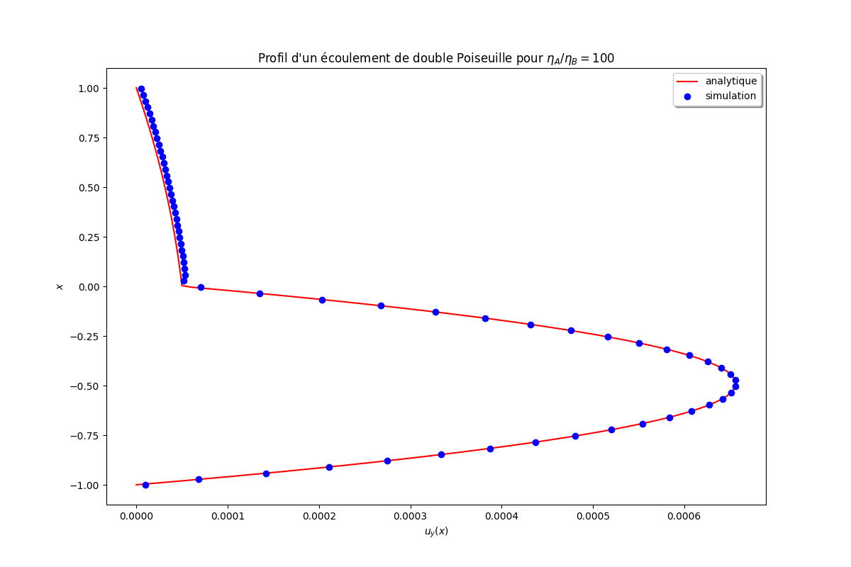
../../_images/Fig_Tuto5_DoublePoiseuille.png — Fig. 49 Comparison between LBM and analytical solution of double-Poiseuille flow

Section author: Alain Cartalade

Implementation of a Navier-Stokes/Cahn-Hilliard model

Objective of this 5th tutorial

1. Create a new kernel `NSCH`

2. Add a new equation in your kernel `NSCH`

3. Modifications inside each file of `NSCH`

4. Verification of your implementation

Table of Contents

Previous topic

Next topic

Implementation of a Navier-Stokes/Cahn-Hilliard model

Objective of this 5th tutorial

1. Create a new kernel NSCH

2. Add a new equation in your kernel NSCH

3. Modifications inside each file of NSCH

4. Verification of your implementation

1. Create a new kernel `NSCH`

2. Add a new equation in your kernel `NSCH`

3. Modifications inside each file of `NSCH`