Implementation of Allen-Cahn coupled with temperature for phase change problems

Objective of this 2nd tutorial

The starting point is the kernel ADE_for_AC-Temp_Tutorial which simulates (again) the Advection-Diffusion Equation (ADE) with the lattice Boltzmann method:

(257)\[\frac{\partial c}{\partial t}+\boldsymbol{\nabla}\cdot(\boldsymbol{u}c)=D\boldsymbol{\nabla}^{2}c\]

Mathematical model

Partial Derivative Equations

In this tutorial we will implement a model to simulate a phase change problem composed of two coupled PDEs, a first one for the evolution of dimensionless temperature:

(258)\[\frac{\partial\theta}{\partial t}=D\boldsymbol{\nabla}^{2}\theta-\frac{\partial\phi}{\partial t}\]

where $\theta$ is a dimensionless temperature, $D$ is the diffusivity parameter and $\phi$ the phase-field. The second equation is for the evolution of phase-field:

(259)\[\frac{\partial\phi}{\partial t}=M_{\phi}\boldsymbol{\nabla}^{2}\phi-\frac{16M_{\phi}}{W^{2}}\phi(1-\phi)(1-2\phi)-\frac{4D}{\mathscr{A}W^{2}}(\theta_{I}-\theta)\phi(1-\phi)\]

where $M_{\phi}$ is the mobility parameter, $W$ is the interface thickness, $\mathscr{A}=10/48$ is known parameter and $\theta_I$ the temperature at interface.

Boundary and initial conditions

The model will be validated with an analytical solution of the 1D Stefan problem which is obtained for Dirichlet boundary conditions.

For temperature equation

The boundary conditions for the temperature equation are:

\[\begin{split}\theta(0,t)&=&\theta_w\\ \theta(L,t)&=&\theta_{\infty}\end{split}\]

where the index $w$ means wall and $L$ is the domain length.

The initial condition is a constant temperature

\[\theta(\boldsymbol{x},0)=\theta_{\infty}\]

For phase-field equation

The boundary conditions for the phase-field equation are:

\[\begin{split}\phi(0,t)&=&0\\ \phi(L,t)&=&1\end{split}\]

The initial condition is a hyperbolic tangent solution at $x_0=0$

\[\phi(\boldsymbol{x},0)=\frac{1}{2}\left[1+\text{tanh}\left(\frac{2(x-x_0)}{W}\right)\right]\]

Objective

In this tutorial we will see how to

add a new equation and all related stages (setup_collider, update, boundary conditions, etc.)
add source terms of Eqs. () and ().

The verification will be carried out with one analytical solution of the Stefan problem (see section 4). We will

compare the outputs of LBM_Saclay with an analytical solution
see the impact of linear and harmonic interpolation of diffusivity $D(\phi)$

1. Create a new kernel `ACT` for Allen-Cahn/Temperature

Make the new kernel ACT in a new folder Allen-Cahn-Temp_Tutorial

That stage 1. is the same than the first tutorial on Cahn-Hilliard.

Copy the folder ADE_for_AC-Temp_Tutorial and rename it Allen-Cahn-Temp_Tutorial

Modify _ADE (for Advection-Diffusion Equation) by _ACT (for Allen-Cahn/Temperature).

2. Add a new equation in your kernel `ACT`

The mathematical model is composed of two coupled PDE. It is necessary to add one supplementary equation.

File Problem_ACT.h

Problem

The number of equation is currently 1

Base::nbEqs = 1;

const int isize = params.isize;
const int jsize = params.jsize;
const int ksize = params.ksize;

Modify it for two equations

Function init_f()

The initialization is currently performed only for one equation:

if (params.collisionType1 == BGK) {
     init1eq<EquationTag1, BGKCollider<dim, npop>>();
} else if (params.collisionType1 == MRT) {
     init1eq<EquationTag1, MRTCollider<dim, npop>>();
}

Add a new block if - else if for EquationTag2

Function update_f()

The update is also performed only for one equation:

if (params.collisionType1 == BGK) {
  update1eq<EquationTag1, BGKCollider<dim, npop>>();
} else if (params.collisionType1 == MRT) {
  update1eq<EquationTag1, MRTCollider<dim, npop>>();
}

Add a new block if - else if for EquationTag2

Function make_boundaries()

The update of bounday conditions is also performed for a single equation

this->bcPerMgr.make_boundaries(scheme.f1, BOUNDARY_EQUATION_1);

Add a new line for f2 and BOUNDARY_EQUATION_2

File LBMScheme_ACT.h

Function struct LBMScheme

Add a new tag tagPHI for EquationTag2

Add two empty functions called setup_collider for EquationTag2 with respectively BGK and MRT collisions

Function make_boundary

The boundary conditions are applied only for Advection-diffusion equation

// ADE boundary
if (Base::params.boundary_types[BOUNDARY_EQUATION_1][faceId] == BC_ANTI_BOUNCE_BACK) {
  real_t boundary_value = Base::params.boundary_values[BOUNDARY_CONCENTRATION][faceId];

  for (int ipop = 0; ipop < npop; ++ipop)
     this->compute_boundary_antibounceback(tagC, faceId, IJK, ipop, boundary_value);
}
else if (Base::params.boundary_types[BOUNDARY_EQUATION_1][faceId] == BC_ZERO_FLUX) {
  for (int ipop = 0; ipop < npop; ++ipop)
     this->compute_boundary_bounceback(tagC, faceId, IJK, ipop, 0.0);
}

Add a new block if - else if for BOUNDARY_EQUATION_2 and tagPHI with keywork BOUNDARY_PHASE_FIELD

3. Modifications inside each file of your kernel `ACT`

Advice

During your implementation, it is strongly recommended to compile regularly to detect any typos. See Advice

File Index_ACT.h

Declaration of new fields

In enum ComponentIndex, only the indices for macroscopic fields such as concentration $c$ (IC) and velocity components $u_x$ (IU), $u_y$ (IV) & $u_z$ (IW) are declared:

enum ComponentIndex {
  IU     , /*!< X velocity / momentum index */
  IV     , /*!< Y velocity / momentum index */
  IW     , /*!< Z velocity / momentum index */
  IC     , /*!< Phase field index */
  COMPONENT_SIZE /*!< invalid index, just counting number of fields */
};

Replace IC by ITEMP and add the new indices for chemical potential IPHI and laplacian IDPHIDT.

Add new outputs

In struct index2names only the strings for concentration and velocity components are written:

map[IC ] = "comp";
map[IU ] = "vx";
map[IV ] = "vy";
map[IW ] = "vz";

Modify for temperature and add new outputs for $\phi$ and $\partial \phi/\partial t$.

File Models_ACT.h

Add specific functions for temperature equation

Add a function Source_TEMP for the source term of temperature equation

Modify the name of collision rate function for temperature equation

Warning

Because IC has been replaced by ITEMP in enum ComponentIndex (file Index_ACT.h), don’t forget to find and replace in all functions lbmState[IC] by lbmState[ITEMP].

Add specific functions for phase-field equation

Add a new function M0_PHI

Add a new function M2_PHI

Add a source term.

Add a new function tau_PHI for collision rate using the mobility $M_\phi$ of Allen-Cahn equation

Add a new hyperbolic tangent function phi0 for initial condition

Read and declare all parameters in ModelParams

The Allen-Cahn equation involves three paramters: the interface thickness $W$ and the mobility $M_\phi$ and the interface temperature $\theta_I$.

Read and declare Allen-Cahn parameters in ModelParams

Add condition for initial condition

Currently only one condition exits for intial condition:

if (initTypeStr == "gaussian") initType = ADE_GAUSSIAN;

Add the necessary condition for one initialization

Solution
if (initTypeStr == "gaussian") initType = ADE_GAUSSIAN;
else if (initTypeStr == "vertical") initType = PHASE_FIELD_INIT_VERTICAL;
Warning

Don’t forget to declare all keywords PHASE_FIELD_INIT_VERTICAL in file InitConditionsTypes.h

File LBMScheme_ACT.h

Function setup_collider with BGK for temperature equation

The function setup_collider is written for solving Advection-Diffusion Equation.

const real_t M0     = Model.M0_TEMP(tagC, lbmState);
const RVect<dim> uc = Model.M1_TEMP<dim>(tagC, lbmState);
const real_t M2     = Model.M2_TEMP(tagC, lbmState);
// ipop = 0
collider.f[0]   = Base::get_f_val(tag, IJK, 0);
collider.S0[0]  = 0.0 ;
collider.feq[0] = w[0]*M0;
// ipop > 0
for (int ipop = 1; ipop < npop; ++ipop) {
  collider.f[ipop]   = this->get_f_val(tag, IJK, ipop);
  collider.S0[ipop]  = 0.0 ;
  collider.feq[ipop] = w[ipop] * (M2 + c_cs2 * Base::compute_scal(ipop, uc));
}

Modify it for the source term.

Function setup_collider with BGK for phase-field equation

The function setup_collider is empty.

void setup_collider(EquationTag2 tag, const IVect<dim>& IJK, BGK_Collider& collider) const
{
}

Inspired with the temperature equation, write your setup_collider.

Function init_macro

After the initialization for ADE_GAUSSIAN:

if (Model.initType == ADE_GAUSSIAN) {
  c  = Model.ampl * exp( - ( SQR(x-Model.x0) / (2 * SQR(Model.sigmax)) + SQR(y-Model.y0) / (2 * SQR(Model.sigmay)) )) ;
  vx = Model.initVX;
  vy = Model.initVY;
}

Write an initial condition corresponding to keywords PHASE_FIELD_INIT_VERTICAL

Save in appropriate arrays

Function update_macro

Currently, only the concentration and the velocity are updated:

const real_t c  = moment_c;
const real_t vx = Model.initVX;
const real_t vy = Model.initVY;

this->set_lbm_val(IJK, IC , c );
this->set_lbm_val(IJK, IU , vx);
this->set_lbm_val(IJK, IV , vy);

Add for phi

Add for dphidt

Save in arrays

Function update_macro_grad

For that phase change model there is no need to compute additional gradient or laplacian.

File InitConditionsTypes.h

Add the keywords of initial conditions

In file InitConditionsTypes.h, two keywords are currently declared:

enum InitCondition{
       PHASE_FIELD_INIT_UNDEFINED,
       ADE_GAUSSIAN
};

Simply add after ADE_GAUSSIAN, the new keyword for Allen-Cahn: PHASE_FIELD_INIT_VERTICAL.

4. Verifications of your implementation

Solution of reference

The LBM implementation is compared with one analytical solution of the Stefan problem. The domain is supposed to be semi-infinite $]0,L]$ (with $L$ big) with Dirichlet boundary conditions $\theta(0,t)=\theta_w$ and $\theta(L,t)=\theta_{\infty}$. The initial condition is $\theta(x,0)=\theta_{\infty}$.

Analytical solution

The analytical solution of this problem gives the interface position $x_i(t)$, the liquid (or solid) temperature $\theta_{l}(x,t)$ and the gas (or liquid) temperature $\theta_{g}(x,t)$. Those solutions depend on a parameter $\xi$ which is given by the transcendental equation.

Interface position

\[x_{i}(t)=2\xi\sqrt{\alpha_{l}t}\]

Liquid temperature

\[\theta_{l}(x,t)=\theta_{w}+(\theta_{I}-\theta_{w})\frac{\mbox{erf}(x/2\sqrt{\alpha_{l}t})}{\mbox{erf}(\xi)}\]

Gas temperature

\[\theta_{g}(x,t)=\theta_{\infty}+(\theta_{I}-\theta_{\infty})\frac{\mbox{erfc}(x/2\sqrt{\alpha_{g}t})}{\mbox{erfc}(\xi\sqrt{\alpha_{l}/\alpha_{g}})}\]

Transcendental equation

\[\frac{e^{-\xi^{2}}}{\mbox{erf}(\xi)}+\left(\frac{\alpha_{g}}{\alpha_{l}}\right)^{1/2}\frac{\theta_{I}-\theta_{\infty}}{\theta_{I}-\theta_{w}}\frac{e^{-\xi^{2}(\alpha_{l}/\alpha_{g})}}{\mbox{erfc}(\xi\sqrt{\alpha_{l}/\alpha_{g}})}=-\frac{\xi\sqrt{\pi}}{\theta_{w}}\]

Input parameters

$\alpha_l$, $\alpha_g$: respectively diffusity of liquid and Gas
$\theta_w$: temperature at left boundary
$\theta_{\infty}$: temperature at right boundary and initial condition
$\theta_I$: temperature at interface

Fortran code and analytical profile

The analytical solution is implemented in a Fortran code. For validating our LBM implementation, the profiles of temperature for liquid (or gas) and solid (or liquid) with the position $x$ are given in two output files T_Liq_Chgt_Phase200000.dat and T_Sol_Chgt_Phase200000.dat. Both files are in the folder case01. After $2\times10^5 \delta t$ the temperature profile is presented on Fig. Fig. 44 for liquid (black) and gas (blue).

Parameters for reference profile

$\theta_w=-0.3$
$\theta_{\infty}=0.3$
$\theta_I=0$
$\alpha_l=\alpha_g=0.1$
$L=500$: length of computational domain
$\delta x=1$: space step
$\delta t=1$: time step
$x_i(0)=0$: interface position at left boundary

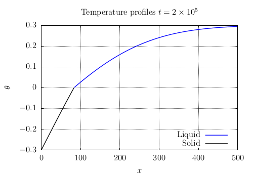
Fig. 44 Temperature profile at $t=2\times 10^5 \delta t$.

Make your input file

Edit your .ini input file

Set appropriate values of [run] section

Set appropriate values of [mesh] section

Set appropriate values of [lbm] section

Set Dirichlet boundary conditions for [equation1] and [equation2].

Set the same input parameters and mobility=0.3 with appropriate value of interface thickness

Set initial condition

Set outputs

Run LBM_Saclay

Run LBM_Saclay with your input datafile

Post-process your results

Results

Generate your csv files with Paraview

In paraview export one temperature profile along x-axis in .csv format (see paraview commands in Run “Two-phase with fluid flows” PART A: Verifications).

Alternatively, your .csv files can generated by using the pvpython command
$ path_to_pvpython/pvpython Profil-Temp.pvpy
where Profil-Temp.pvpy is in

Superpose with Gnuplot

A gnuplot script Profil_Comparison_Analy-LBM.gnutex is also available in the folder
$ gnuplot Profil_Comparison_Analy-LBM.gnutex
will generate a new file Profile-Temp-Stefan_LBM-Analytical.tex
$ pdflatex Profile-Temp-Stefan_LBM-Analytical.tex
to make the pdf file. You should obtain Fig. Fig. 45

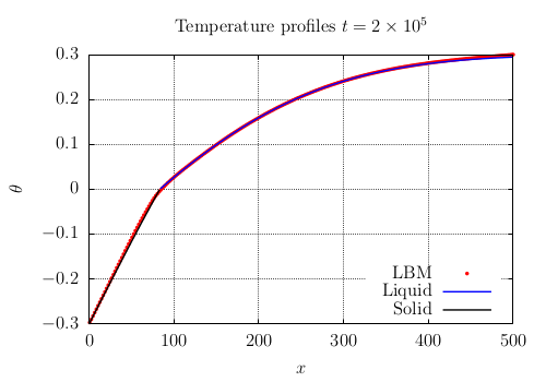
Fig. 45 Comparison between LBM and analytical solution² at $t=2\times 10^5 \delta t$.

Different diffusivities

Case $D_l \neq D_g$

Modify your kernel in order to interpolate the diffusivity in the temperature equation by $D(\phi)=(1-\phi)D_l+\phi D_g$ where $D_l$ and $D_g$ are respectively the thermal diffusivity in liquid and gas. Keep $D=1$ in the source term of phase-field equation.

Add necesary values of $D_l$ and $D_g$ in your the .ini input file
Superpose with analytical solution with $D_l=0.14$ and $D_g=0.014$
Use the harmonic interpolation for $D(\phi)$ for temperature equation and keep $D=1$ in phase-field equation. Compare with analytical solution.

Compare the impact on curves

Solution

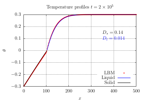
Fig. 46 Comparison between LBM and analytical solution at $t=2\times 10^5 \delta t$ for $D_l=0.14$ and $D_g=0.014$.

Section author: Alain Cartalade

Implementation of Allen-Cahn coupled with temperature for phase change problems

Objective of this 2nd tutorial

1. Create a new kernel `ACT` for Allen-Cahn/Temperature

2. Add a new equation in your kernel `ACT`

3. Modifications inside each file of your kernel `ACT`

4. Verifications of your implementation

Table of Contents

Previous topic

Next topic

Implementation of Allen-Cahn coupled with temperature for phase change problems

Objective of this 2nd tutorial

1. Create a new kernel ACT for Allen-Cahn/Temperature

2. Add a new equation in your kernel ACT

3. Modifications inside each file of your kernel ACT

4. Verifications of your implementation

1. Create a new kernel `ACT` for Allen-Cahn/Temperature

2. Add a new equation in your kernel `ACT`

3. Modifications inside each file of your kernel `ACT`