Overview of Lattice Boltzmann Methods

This part is a quick introduction to the Lattice Boltzmann Method. More details on the origin and the theoretical aspects of the method can be found in reference [1].

More details of numerical methods that are implemented in LBM_Saclay will be found in the pages below.

Continuous Boltzmann equation

At mesoscopic level, a collection of particles can be described by a distribution function of particles \(f(\boldsymbol{x},\boldsymbol{c},t)\) which is a function of position \(\boldsymbol{x}\), microscopic speeds \(\boldsymbol{c}\) and time \(t\). Its evolution in time and space obeys to the continuous Boltzmann equation:

(339)\[\frac{\partial f}{\partial t}+\boldsymbol{c}\cdot\boldsymbol{\nabla}f+\boldsymbol{F}\cdot\boldsymbol{\nabla}_{\boldsymbol{c}}f=\Omega(f,f^{eq})\label{eq:Boltzmann_Eq}\]

which is a transport equation where \(\boldsymbol{F}\) is the external force and \(\Omega(f,f^{eq})\) is the collision operator that relaxes the distribution function \(f\) toward an equilibrium \(f^{eq}\). For the classical Batnaghar-Gross-Krook (BGK) approximation, that collision operator simply writes:

(340)\[ \Omega(f,f^{eq})\sim-\frac{1}{\lambda}\left[f-f^{eq}\right]\]

where \(\lambda\) is the collision time. Eq. (339), computes the evolution of the distribution function \(f\) in space and time. The macrosopic quantities such as the density \(\rho\), impulsion \(\rho\boldsymbol{u}\) and energy \(\rho\varepsilon\) can be derived from that distribution function by integration over the velocity space:

\[\begin{split}\begin{aligned} \rho & =\int fd\boldsymbol{c}\\ \rho\boldsymbol{u} & =\int f\boldsymbol{c}d\boldsymbol{c}\\ \rho\varepsilon & =\frac{1}{2}\int(\boldsymbol{c}-\boldsymbol{u})^{2}fd\boldsymbol{c}\end{aligned}\end{split}\]

Those macroscopic quantities are called the moments of the distribution function \(f(\boldsymbol{x},\boldsymbol{c},t)\).

For more details on the origin of the Boltzmann equation and the physical interpretation of distribution function see reference [2].

Discretization of velocity space

Eq. (339) must be discretized for \(\boldsymbol{x}\), \(\boldsymbol{c}\) and \(t\). After discretization of the velocity space with a finite number of speeds, \(\boldsymbol{c}\) becomes \(\boldsymbol{c}_i\) where \(i\) is the index of velocity varying between \(0\) and the total number of speeds \(N\). The discrete distribution function \(f(\boldsymbol{x},\boldsymbol{c}_i,t)\) is noted \(f_i(\boldsymbol{x},t)\).

Discrete velocity space

The discrete velocity is related to them time-step \(\delta t\) and space-step of spatial discretization \(\delta x\) by

(341)\[\boldsymbol{c}_i = \frac{\delta x}{\delta t}\boldsymbol{e}_i\]

where \(\boldsymbol{e}_i\) are the moving directions. A representation of that discretization is presented on Fig. 1. On that example, for one position \(\boldsymbol{x}\) and time \(t\), the distribution function \(f\) represents a collection of particles of different velocities. After discretization of \(\boldsymbol{c}\), only five speeds are kept on that example: right-direction (blue), upward-direction (red), left-direction (green), downward-direction (orange) and non-moving direction (black).

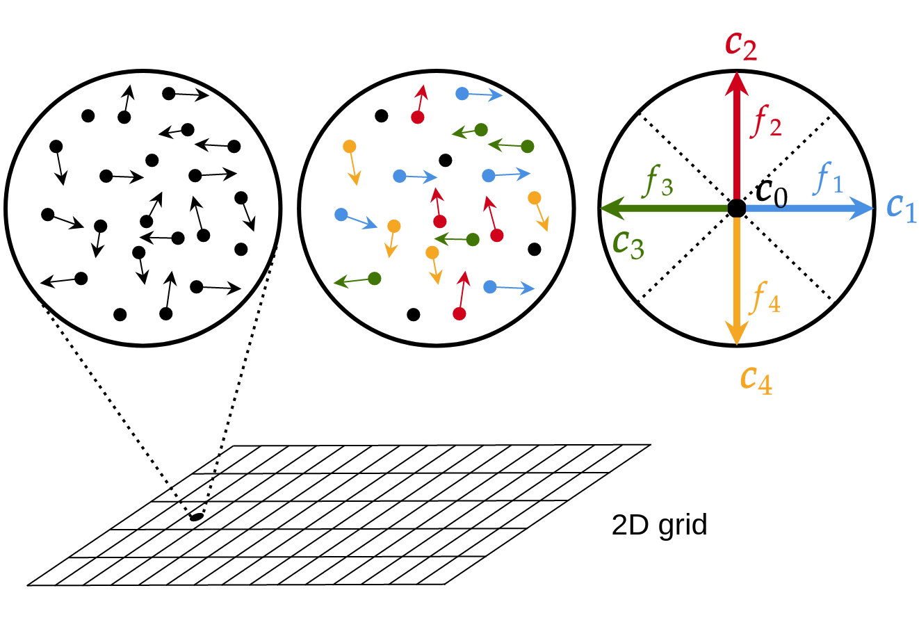
Fig. 41 Fig. 1: Principle of discrete velocity space and discrete distribution function \(f_i\)

After discretization in space the lattice is a superposition of one standard mesh with the discrete velocity space. If the dimension of space is 2 and the number of total discrete speeds is 5, the lattice name D2Q5 is presented on Fig. 2.

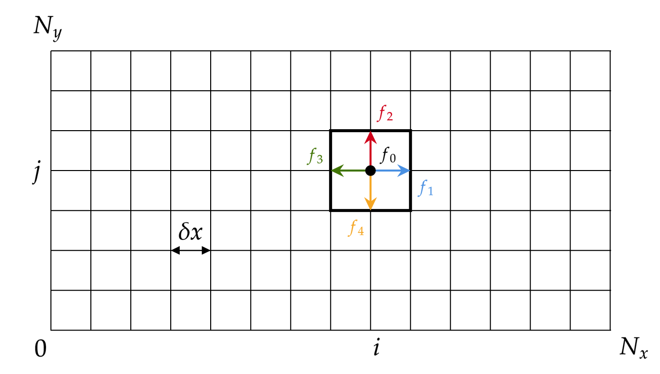
Fig. 42 Fig. 2: Example of lattice D2Q5 after discretization of \(\boldsymbol{x}\) and \(\boldsymbol{c}\).

Lattices

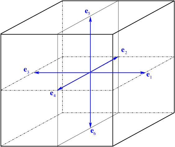
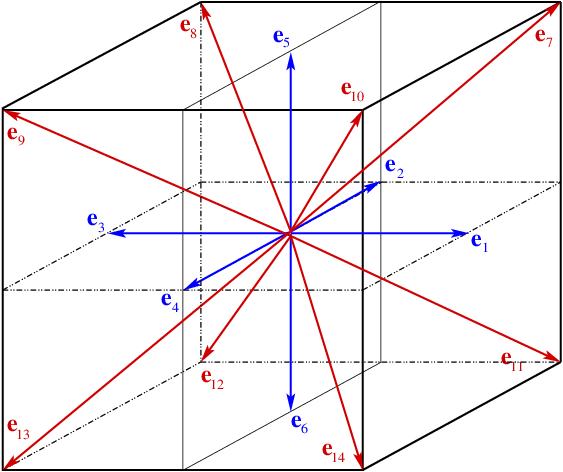
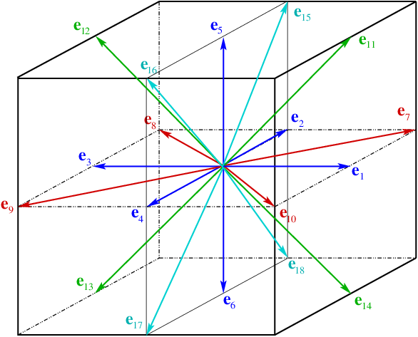
Many lattices exist in LBM. The most popular lattices are D2Q9 for two-dimensional simulations, and D3Q15, D3Q19 and D3Q27 for three-dimensional simulations. Let us mention that for simulations problems involving only diffusion, the minimal lattices D2Q5 and D3Q7 can be sufficient. In LBM_Saclay, one supplementary lattice is available: D3Q27.

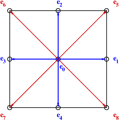
Two-dimensional lattices: D2Q5 (left) and D2Q9 (right)

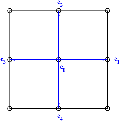
For lattice D2Q5, the five moving vectors are defined by

(342)\[\begin{split}\boldsymbol{e}_{0}=\left(\begin{array}{c} 0\\ 0 \end{array}\right),\quad\boldsymbol{e}_{1}=\left(\begin{array}{c} 1\\ 0 \end{array}\right),\quad\boldsymbol{e}_{2}=\left(\begin{array}{c} 0\\ 1 \end{array}\right),\quad\boldsymbol{e}_{3}=\left(\begin{array}{c} -1\\ 0 \end{array}\right),\quad\boldsymbol{e}_{4}=\left(\begin{array}{c} 0\\ -1 \end{array}\right)\end{split}\]

For D2Q9, the four diagonal moving vectors are added:

(343)\[\begin{split}\boldsymbol{e}_{5}=\left(\begin{array}{c} 1\\ 1 \end{array}\right),\quad\boldsymbol{e}_{6}=\left(\begin{array}{c} -1\\ 1 \end{array}\right),\quad\boldsymbol{e}_{7}=\left(\begin{array}{c} -1\\ -1 \end{array}\right),\quad\boldsymbol{e}_{8}=\left(\begin{array}{c} 1\\ -1 \end{array}\right)\end{split}\]

Three-dimensional lattices

Fig. 43 Lattice D3Q7

Fig. 44 Lattice D3Q15

Fig. 45 Lattice D3Q19

Lattice Boltzmann Equation (LBE)

Once the Boltzmann equation is discretized in space and time the following Lattice Boltzmann Equation (LBE) is obtained:

(344)\[f_{i}(\boldsymbol{x}+\boldsymbol{c}_{i}\delta t,t+\delta t)=f_{i}(\boldsymbol{x},t)-\frac{1}{\tau}\left[f_{i}(\boldsymbol{x},t)-f_{i}^{eq}(\boldsymbol{x},t)\right]\]

where \(\delta t\) is the time step and the second term of the right-hand side is the discrete BGK collision operator. The coefficient of proportionnality \(\tau\) is the collision rate which is related to the collision time by

(345)\[\tau=\frac{\lambda}{\delta t}\]

The right-hand side represents the collision stage and it is often noted

(346)\[f_{i}^{\star}(\boldsymbol{x},t)=f_{i}(\boldsymbol{x},t)-\frac{1}{\tau}\left[f_{i}(\boldsymbol{x},t)-f_{i}^{eq}(\boldsymbol{x},t)\right]\]

The expression of the equilibrium distribution function \(f_i^{eq}\) depends on the physical problem to simulate.

Equilibrium distribution function

For low Mach version of Navier-Stokes equations

For example for low Mach version of Navier-Stokes equations:

(347)\[f_{i}^{eq}(\boldsymbol{x},t)=w_{i}\rho\left[1+\frac{\boldsymbol{c}_{i}\cdot\boldsymbol{u}}{c_{s}^{2}}+\frac{(\boldsymbol{c}_{i}\cdot\boldsymbol{u})^{2}}{2c_{s}^{4}}-\frac{\boldsymbol{u}\cdot\boldsymbol{u}}{2c_{s}^{2}}\right]\]

where the coefficient \(c_{s}\), called the sound speed, is defined by

(348)\[c_{s}=\frac{1}{\sqrt{3}}\frac{\delta x}{\delta t}\]

and \(w_{i}\) are weights which depend on the lattice considered.

For Advection-Diffusion Equation (ADE)

(349)\[f_{i}^{eq}(\boldsymbol{x},t)=w_{i}T\left[1+\frac{\boldsymbol{u}\cdot\boldsymbol{c}_{i}}{c_{s}^{2}}\right]\]

Explicit algorithm

The algorithm is extremely simple and it can be summarized into three main stages:

1. Collision: \(f_{i}(\boldsymbol{x},t)\rightarrow f_{i}^{\star}(\boldsymbol{x},t)\) (right-hand side of Eq. (344))

2. Streaming: \(f_{i}^{\star}(\boldsymbol{x},t)\rightarrow f_{i}(\boldsymbol{x}+\boldsymbol{c}_{i}\delta t,t+\delta t)\) (left-hand side)

3. Update the density and impulsion

(350)\[\rho(\boldsymbol{x},t)=\sum_{i}f_{i}(\boldsymbol{x},t)\]

(351)\[\rho(\boldsymbol{x},t)\boldsymbol{u}(\boldsymbol{x},t)=\sum_{i}f_{i}(\boldsymbol{x},t)\boldsymbol{c}_{i}\]

Algorithm

Finally, once the lattice is defined, the Navier-Stokes solver using the lattice Boltzmann method consists in a succession of collision and streaming:

(352)\[f_{i}(\boldsymbol{x}+\boldsymbol{c}_{i}\delta t,t+\delta t)=f_{i}(\boldsymbol{x},t)-\frac{1}{\tau}\left[f_{i}(\boldsymbol{x},t)-f_{i}^{eq}(\boldsymbol{x},t)\right]\]

where the equilibrium distribution function is defined by

(353)\[f_{i}^{eq}(\boldsymbol{x},t)=w_{i}\rho\left[1+\frac{\boldsymbol{c}_{i}\cdot\boldsymbol{u}}{c_{s}^{2}}+\frac{(\boldsymbol{c}_{i}\cdot\boldsymbol{u})^{2}}{2c_{s}^{4}}-\frac{\boldsymbol{u}\cdot\boldsymbol{u}}{2c_{s}^{2}}\right]\]

Once those two stages are performed, the density and impulsion are updated with the relationships:

(354)\[\rho(\boldsymbol{x},t)=\sum_{i}f_{i}(\boldsymbol{x},t)\]

(355)\[\rho(\boldsymbol{x},t)\boldsymbol{u}(\boldsymbol{x},t)=\sum_{i}f_{i}(\boldsymbol{x},t)\boldsymbol{c}_{i}\]

Chapman-Enskog expansion

The link between the discrete Boltzmann equation with the macroscopic Navier-Stokes equations is performed with a mathematical procedure of asymptotic expansions called the Chapman-Enskog expansion. Details of those expansions can be founds in the link below.

• Chapman-Enskog expansion for Navier-Stokes equations

The starting point is the algorithm Eq. (344) – (355). Once the Chapman-Enskog expansion is performed, the procedure recovers the following macroscopic equations:

Equivalent macroscopic PDE with the condition \(\bigl|\boldsymbol{u}\bigr|\ll c_{s}\)

(398)\[\partial_{t}\rho+\boldsymbol{\nabla}\cdot(\rho\boldsymbol{u})=0\]

for the mass balance equation, and

(399)\[\partial_{t}(\rho\boldsymbol{u})+\boldsymbol{\nabla}\cdot(\rho\boldsymbol{u}\boldsymbol{u})=-\boldsymbol{\nabla}p+\boldsymbol{\nabla}\cdot\left[\rho\nu(\boldsymbol{\nabla}\boldsymbol{u}+(\boldsymbol{\nabla}\boldsymbol{u})^{T})\right]+\mathcal{O}(\rho u^{3})\]

where the pressure is given by the law of perfect gas \(p=\rho c_{s}^{2}\) and the kinematic viscosity \(\nu\) is related to the relaxation rate \(\tau\) by \(\nu=(\tau-1/2)c_{s}^{2}\delta t\).

Variable change in LBE with a source term

• Variable change in LBE for source term

Bibliography

[1]

Krüger T., H. Kusumaatmaja, A. Kuzmin, O. Shardt, G. Silva, E. Viggen, The Lattice Boltzmann Method: Principles and Practice, Graduate Texts in Physics, Springer, 2016.

[2]

Bird G.A., Molecular Gas Dynamics and the Direct Simulation of Gas Flows, Oxford Engineering Science Series, 1994.

Section author: Alain Cartalade