Model of Navier-Stokes/Korteweg (NSK)

The Navier-Stokes/Korteweg model (NSK) is a popular alternative model for simulating two-phase flows without introducing a phase-field \(\phi\). That model is a low Mach formulation of the Navier-Stokes equations, where \(\rho\) plays the role of phase index. The two-phase behavior is obtained by an appropriate choice of the Equation of State (EoS).

Mathematical model of van der Waals fluids

Model of Navier-Stokes/Korteweg

The mathematical model is based on the low Mach formulation of the Navier-Stokes equations. The mass balance writes

(84)\[\frac{\partial\rho}{\partial t}+\boldsymbol{\nabla}\cdot(\rho\boldsymbol{u})=0\]

The impulsion balance equation makes appear the pressure tensor

(85)\[\frac{\partial(\rho\boldsymbol{u})}{\partial t}+\boldsymbol{\nabla}\cdot(\rho\boldsymbol{u}\boldsymbol{u})=-\boldsymbol{\nabla}\cdot\overline{\overline{\boldsymbol{P}}}+\boldsymbol{\nabla}\cdot\left[\eta\left(\boldsymbol{\nabla}\boldsymbol{u}+\boldsymbol{\nabla}\boldsymbol{u}^{T}\right)\right]\]

where \(\overline{\overline{\boldsymbol{P}}}\) is the pressure tensor which is defined by

(86)\[\overline{\overline{\boldsymbol{P}}}=\left[p^{eos}(\rho,T)-\kappa\rho\boldsymbol{\nabla}^{2}\rho-\frac{1}{2}\kappa\bigl|\boldsymbol{\nabla}\rho\bigr|^{2}\right]\overline{\overline{\boldsymbol{I}}}+\kappa\boldsymbol{\nabla}\rho\otimes\boldsymbol{\nabla}\rho\]

In Eq. (572) \(p^{eos}(\rho,T)\) is the thermodynamic pressure defined from the potential by:

(101)\[p^{eos}(\rho)=\rho\partial_{\rho}\mathcal{W}(\rho)-\mathcal{W}(\rho)\]

The thermodynamic pressure is a function of density \(\rho\) and temperature \(T\).

Equations of state (EoS)

Several Equations of State (EoS) exist in the literature to simulate two-phase flows: Van der Waals, Carnahan-Starling, Peng-Robinson, Redlich-Kwong, etc. Only the first two have been tested in LBM_Saclay.

Van der Waals EoS

The Van der Waal EoS writes

(88)\[p_{vdW}^{eos}(\rho,T_k)=\frac{\rho RT_k}{1-b\rho}-a\rho^{2}\]

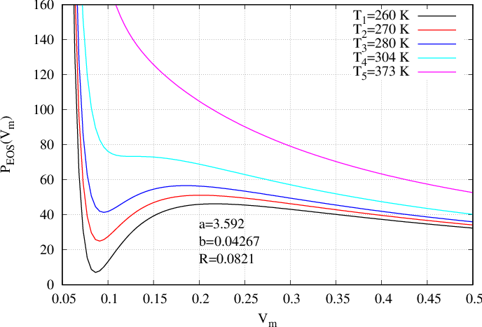
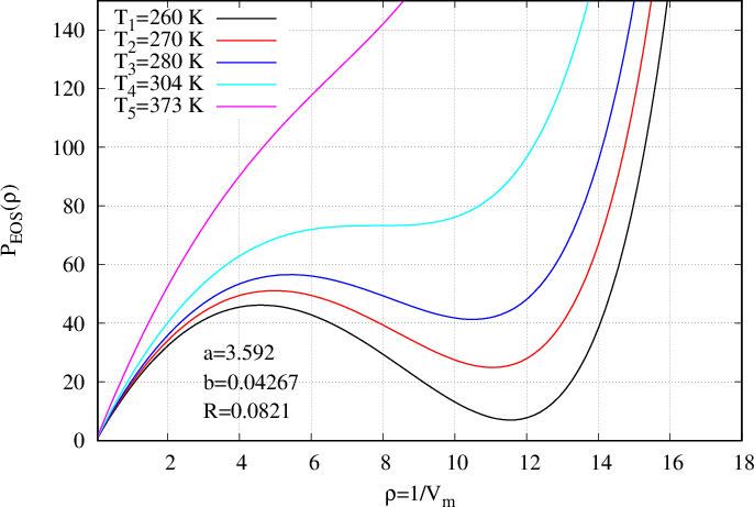
where \(T_k\) is a constant temperature which must be indicated in the input file as well as the two coefficients \(a,b\) and the constant of perfect gas \(R\). Such an equation of state is presented in Fig. 38 for five different temperatures (subscript \(k=1,...,5\)). That EoS can be derived from a thermodynamic potential (101) where \(\mathcal{W}_{vdW}\) is defined by

(89)\[\mathcal{W}_{vdW}(\rho)=\rho RT_{k}\ln\left(\frac{\rho}{1-b\rho}\right)-a\rho^{2}\]

Finally the chemical potential \(\mu_{\rho}\) is derived by the Euler-Lagrange equation \(\mu_{\rho}=\mathcal{W}^{\prime}(\rho)-\kappa\boldsymbol{\nabla}^{2}\rho\):

(90)\[\mu_{\rho}^{vdW}=RT_k\left[\ln\left(\frac{\rho}{1-b\rho}\right)+\frac{1}{1-b\rho}\right]-2a\rho-\kappa\boldsymbol{\nabla}^{2}\rho\]

On Fig. 37 the pressure is presented as a function of volume \(V\) whereas on Fig. 38 it is presented as a function of density \(\rho\). On those figures, one temperature \(T_5\) (the magenta curve) is above the critical temperature. The curve is monotonous and only one density corresponds to one pressure. For temperature \(T_4\) (cyan curve) there is an inflexion point corresponding to the critical temperature (zero derivative with respect to rho). At last, for three next temperatures \(T_1,T_2,T_3\) (respectively black, red and blue curves), the pressure presents a cubic form enabling the existence of two densities corresponding to one pressure.

Fig. 37 Phase diagram \(P-V\)

Fig. 38 Phase diagram \(P-\rho\)

Carnahan-Starling EoS

One improvement of the vdW EoS is the Carnahan-Starling EoS which writes:

(91)\[p_{CS}^{eos}(\rho,T)=\rho RT\frac{1+b\rho/4+(b\rho/4)^{2}-(b\rho/4)^{3}}{(1-b\rho/4)^{3}}-a\rho^{2}\]

where, once again, the input parameters are \(R,T,a,b\). That EoS can be derived from the potential:

(92)\[\mathcal{W}_{CS}(\rho)=\rho RT\left[\frac{3-b\rho/2}{(1-b\rho/4)^{2}}+\ln(b\rho/4)\right]-a\rho^{2}\]

Finally, the chemical potential writes:

(93)\[\mu_{\rho}^{CS}=RT\left[\frac{3-b\rho/4}{(1-b\rho/4)^{3}}+\ln(b\rho/4)+1\right]-2a\rho-\kappa\boldsymbol{\nabla}^{2}\rho\]

Two other popular EoS exist in the literature. We only mention them here. They could be tested in the future in LBM_Saclay.

Redlich-Kwong (RK)

(94)\[\begin{split}p_{RK}^{eos}(\rho,T)&=\frac{\rho RT}{1-b\rho}-\frac{a\alpha(T)\rho^{2}}{1+b\rho}\\\alpha(T)&=1/\sqrt{T}\\\text{Soave modif }\alpha(T)&=[1+(\alpha_{1}+\alpha_{2}\omega-\alpha_{3}\omega^{2})(1-\sqrt{T/T_{c}})]^{2}\\\text{coeff}&\alpha_{1}=0.480,\quad\alpha_{2}=1.574,\quad\alpha_{3}=0.176\end{split}\]

Peng-Robinson (PR)

(95)\[\begin{split}p_{PR}^{eos}(\rho,T)&=\frac{\rho RT}{1-b\rho}-\frac{a\alpha(T)\rho^{2}}{1+2b\rho-b^{2}\rho^{2}}\\\alpha(T)&=[1+(\alpha_{1}+\alpha_{2}\omega+\alpha_{3}\omega^{2})(1-\sqrt{T/T_{c}})]^{2}\\\text{coeff}&\alpha_{1}=0.37464,\quad\alpha_{2}=1.54226,\quad\alpha_{3}=0.26992\end{split}\]

Equivalence of tensor pressure

In most of numerical methods that implement the NSK model, the pressure tensor Eq. (572) is not directly discretized because there exist two equivalent algebraic forms which are easier to implement. The first one is the potential form and the second involves the chemical potential.

First form: potential form

(96)\[-\boldsymbol{\nabla}\cdot\overline{\overline{\boldsymbol{P}}}=-\boldsymbol{\nabla}p^{eos}+\boldsymbol{F}\]

with

(97)\[\boldsymbol{F}=\kappa\rho\boldsymbol{\nabla}(\boldsymbol{\nabla}^{2}\rho)\]

Demo:

\[\begin{split}\partial_{\beta}P_{\alpha\beta}&=\partial_{\beta}\left\{ \left[p^{eos}-\kappa\rho\partial_{\gamma}\partial_{\gamma}\rho-\frac{1}{2}\kappa(\partial_{\gamma}\rho)^{2}\right]\delta_{\alpha\beta}+\kappa(\partial_{\alpha}\rho)(\partial_{\beta}\rho)\right\} \\&=\partial_{\alpha}p^{eos}-\partial_{\alpha}(\kappa\rho\partial_{\gamma}\partial_{\gamma}\rho)-\frac{1}{2}\underbrace{\partial_{\alpha}(\kappa(\partial_{\gamma}\rho)^{2})}_{\text{development}}+\underbrace{\partial_{\gamma}(\kappa(\partial_{\alpha}\rho)(\partial_{\gamma}\rho))}_{\text{index }\beta\rightarrow\gamma}\\&=\partial_{\alpha}p^{eos}-\partial_{\alpha}(\kappa\rho\partial_{\gamma}\partial_{\gamma}\rho)-\left[\kappa(\partial_{\gamma}\rho)(\partial_{\alpha}\partial_{\gamma}\rho)\right]+\underbrace{\partial_{\gamma}(\kappa(\partial_{\alpha}\rho)(\partial_{\gamma}\rho))}_{\text{Development}}\\&=\partial_{\alpha}p^{eos}-\underbrace{\partial_{\alpha}(\kappa\rho\partial_{\gamma}\partial_{\gamma}\rho)}_{\text{Development}}-\left[\cancel{\kappa(\partial_{\gamma}\rho)(\partial_{\alpha}\partial_{\gamma}\rho)}\right]+\left[\cancel{\kappa\partial_{\gamma}(\partial_{\alpha}\rho)(\partial_{\gamma}\rho)}+\kappa(\partial_{\alpha}\rho)\partial_{\gamma}(\partial_{\gamma}\rho)\right]\\&=\partial_{\alpha}p^{eos}-\left[\bcancel{\kappa(\partial_{\alpha}\rho)\partial_{\gamma}\partial_{\gamma}\rho}+\kappa\rho\partial_{\alpha}\partial_{\gamma}\partial_{\gamma}\rho\right]+\bcancel{\kappa(\partial_{\alpha}\rho)\partial_{\gamma}(\partial_{\gamma}\rho)}\\&=\partial_{\alpha}p^{eos}-\kappa\rho\partial_{\alpha}(\partial_{\gamma}\partial_{\gamma}\rho)\end{split}\]

Second form: chemical potential form

(98)\[-\boldsymbol{\nabla}\cdot\overline{\overline{\boldsymbol{P}}}=-\rho\boldsymbol{\nabla}\mu_{\rho}\]

with

(99)\[\mu_{\rho}=\mathcal{W}^{\prime}(\rho)-\kappa\boldsymbol{\nabla}^{2}\rho\]

Demo

(100)\[\mu_{\rho}=\mathcal{W}^{\prime}(\rho)-\kappa\boldsymbol{\nabla}^{2}\rho\]

(101)\[p^{eos}(\rho)=\rho\mathcal{W}^{\prime}(\rho)-\mathcal{W}(\rho)\]

\[\begin{split}\rho\boldsymbol{\nabla}\mu_{\rho}&=\rho\boldsymbol{\nabla}\left[\frac{1}{\rho}\left(p^{eos}+\mathcal{W}(\rho)\right)-\kappa\boldsymbol{\nabla}^{2}\rho\right]\\&=\left(p^{eos}+\mathcal{W}(\rho)\right)\rho\boldsymbol{\nabla}\left(\frac{1}{\rho}\right)+\boldsymbol{\nabla}\left(p^{eos}+\mathcal{W}(\rho)\right){\color{gray}-\rho\kappa\boldsymbol{\nabla}(\boldsymbol{\nabla}^{2}\rho)}\\&=\left(p^{eos}+\mathcal{W}(\rho)\right)\cancel{\rho}\left(-\frac{1}{\rho^{\cancel{2}}}\right)\boldsymbol{\nabla}\rho+\boldsymbol{\nabla}p^{eos}+\mathcal{W}^{\prime}(\rho)\boldsymbol{\nabla}\rho{\color{gray}-\rho\kappa\boldsymbol{\nabla}(\boldsymbol{\nabla}^{2}\rho)}\\&=\bigl[-p^{eos}\underbrace{-\mathcal{W}(\rho)+\rho\mathcal{W}^{\prime}(\rho)}_{\equiv+p^{eos}}\bigr]\frac{\boldsymbol{\nabla}\rho}{\rho}{\color{gray}+\boldsymbol{\nabla}p^{eos}-\rho\kappa\boldsymbol{\nabla}(\boldsymbol{\nabla}^{2}\rho)}\\&=\boldsymbol{\nabla}p^{eos}-\rho\kappa\boldsymbol{\nabla}(\boldsymbol{\nabla}^{2}\rho)\end{split}\]

Section author: Alain Cartalade