Model of Navier-Stokes/CAC with surfactant

We detail here the model of two-phase flows with surfactant. Compared to the kernel NSAC_Comp, the equations of mass balance, impulsion balance and levelset are identical. The modification appears in the composition equation.

Mathematical model of two-phase with surfactant

The mathematical model is composed of incompressible Navier-Stokes equations coupled with the phase-field equation and the composition equation. Compared to the NSAC_Comp kernel, the composition equation is modified with a counter term to impose an equilibrium profile at the interface. The model writes as follows.

Mathematical model

Mass balance equation

The mass balance writes:

(53)\[\boldsymbol{\nabla}\cdot\boldsymbol{u}=0\]

where \(\boldsymbol{u}\equiv\boldsymbol{u}(\boldsymbol{x},t)=(u_x,u_y,u_z)^T\) is the fluid velocity.

Impulsion balance equation

The impulsion balance equation writes:

(54)\[\varrho(\phi,c)\left[\frac{\partial\boldsymbol{u}}{\partial t}+\boldsymbol{\nabla}\cdot(\boldsymbol{u}\boldsymbol{u})\right]=-\boldsymbol{\nabla}p_{h}+\boldsymbol{\nabla}\cdot\left[\eta(\phi)\left(\boldsymbol{\nabla}\boldsymbol{u}+\boldsymbol{\nabla}\boldsymbol{u}^{T}\right)\right]+\boldsymbol{F}_{tot}\]

where \(p_{h}\equiv p_{h}(\boldsymbol{x},t)\) is the hydrodynamic pressure, \(\varrho\) is the total densiy and \(\eta\) is the dynamic viscosity. Those quantities are obtained from the interpolation of bulk properties with the phase-field \(\phi\). Their expressions will be given in the subsection “Closure”.

Phase-field equation

The interface is followed by an additional PDE on the phase-field:

(55)\[\frac{\partial\phi}{\partial t}+\boldsymbol{\nabla}\cdot(\boldsymbol{u}\phi)=\boldsymbol{\nabla}\cdot\left[M_{\phi}\left(\boldsymbol{\nabla}\phi-\frac{4}{W}\phi(1-\phi)\boldsymbol{n}_{\phi}\right)\right]\]

where \(\phi\equiv\phi(\boldsymbol{x},t)\) is the phase-field, \(M_{\phi}\) is the mobility and \(W\) is the interface width. That equation is called “Conservative Allen-Cahn” equation (CAC). It is also encountered in the literature as the “Levelset” equation.

Finally, the composition equation is also considered in that model:

Composition equation

(56)\[\frac{\partial c}{\partial t}+\boldsymbol{\nabla}\cdot\left(c\boldsymbol{u}\right)=\boldsymbol{\nabla}\cdot\left[M_{c}\left(\boldsymbol{\nabla} c-c(1-c)\mathcal{P}(\phi)\boldsymbol{n}_{\phi}\right)\right]\]

where \(c\equiv c(\boldsymbol{x},t)\) is the composition, \(M_c\) is the diffusion coefficient and \(\mathcal{P}(\phi)\) is an interpolation polynom defined by

(57)\[\mathcal{P}(\phi)=\beta\frac{4}{W}\phi(1-\phi)\left(1-2\phi\right)\left[\frac{k}{2}+\frac{16}{W²}\epsilon(1-\phi)\phi\right]\]

where \(\beta\), \(k\), and \(\epsilon\) are three coefficients which control the composition height at the interface.

Force and source terms

Force and source terms

The forces are still the same than those defined in NSAC_Comp kernel.

Total force

The total force \(\boldsymbol{F}_{tot}\) in Eq. (54) is defined by

(58)\[\boldsymbol{F}_{tot}=\boldsymbol{F}_{c}+\boldsymbol{F}_{g}+\boldsymbol{F}_{M}\]

where \(\boldsymbol{F}_{c}\) is the capillary force, \(\boldsymbol{F}_{g}\) is the gravity force and \(\boldsymbol{F}_{M}\) is the Marangoni force. They are detailed below.

Gravity force

The gravity force is defined by

(59)\[\boldsymbol{F}_{g}=\varrho(\phi,c)\boldsymbol{g}\]

Capillary force

The capillary force defined by

(60)\[\boldsymbol{F}_{c}=\mu_{\phi}\boldsymbol{\nabla}\phi\]

where the chemical potential \(\mu_{\phi}\) is defined by

(61)\[\mu_{\phi}=\frac{3}{2}\textcolor{red}{\sigma(c)}\left[\frac{16}{W}\phi(1-\phi)(1-2\phi)-W\boldsymbol{\nabla}^{2}\phi\right]\]

Marangoni force

The Marangoni force is defined by

(62)\[\boldsymbol{F}_{M}=\frac{3W}{2}\left[\boldsymbol{\nabla}\textcolor{red}{\sigma(c)}|\boldsymbol{\nabla}\phi|^{2}-\boldsymbol{\nabla}\phi(\boldsymbol{\nabla}\phi\cdot\boldsymbol{\nabla}\textcolor{red}{\sigma(c)})\right]\]

where \(W\) is the interface width and \(\textcolor{red}{\sigma(c)}\) is the surface tension varying with composition \(c\). Two phenomenological laws are given on the next tab-item.

Source term of Eq. (55)

In the last term of the righ-hand side of Eq. (55), the source term \(\mathscr{S}_{\phi}\) can be defined for phase-change problems. In that case, the \(\lambda\) coefficient must be appropriately chosen. For two immiscible fluid flows, that coefficient is set equal to zero.

Phenomenological laws for \(\sigma\)

Phenomenological laws for surface tension

Two models are implemented to modify the surface tension \(\sigma (c)\) with composition \(c\). The first one writes:

(63)\[\sigma(c)=\sigma_{ref}+\frac{d\sigma}{dc}(c-c_{ref})\]

In that case we need to set the option Closure_Model=0 and disgmadcomp is used in the .ini file:

(64)\[\frac{d\sigma}{dc}=\sigma_{c}<0\]

For simulations of two-phase with surfactant, another law between the surface tension and the composition is used:

(65)\[\sigma=\sigma_{0}\left(1+\gamma ln\left(1-c\right)\right)\]

in that case, option Closure_Model=1 must be set and the coefficient \(\gamma\) is named beta_log in .ini file and \(\sigma_{0}\) are two coefficients to be indicated inside the .ini file.

Closure relationships

In order to close the model, it is required to add closure relationships. The total density \(\varrho\) is interpolated by \(\phi\) and \(c\):

(66)\[\varrho(\phi,c)=\rho_{1}(c)p(\phi)+\rho_{0}(c)(1-p(\phi))\]

where each bulk density \(\rho_{\Phi}\) is linearly interpolated by \(c\):

(67)\[\rho_{\Phi}(c)=(\rho_{\Phi}^{eq}-\rho_{\Phi}^{ini})\frac{c-c_{\Phi}^{ini}}{c_{\Phi}^{eq}-c_{\Phi}^{ini}}+\rho_{\Phi}^{ini}\]

The index \(\Phi=0,1\) indicates phase 0 or phase 1. The interpolation function \(p(\phi)\) can be chosen:

(68)\[\begin{split}p(\phi)=\begin{cases} \phi\qquad\text{or}\\ \phi^{2}(3-2\phi) \end{cases}\end{split}\]

The dynamic viscosity is interpolated by a harmonic mean formula:

(69)\[\frac{1}{\eta(\phi)}=\frac{\phi}{\eta_{1}}+\frac{1-\phi}{\eta_{0}}\]

Finally in the composition equation, the diffusion parameter is also linearly interpolated:

(70)\[\mathcal{D}(\phi)=D_{1}\phi+D_{0}(1-\phi)\]

List of input parameters in .ini file

Section [lbm]

In section [lbm] use the keyword problem=NSAC_Comp to simulate that mathematical model. Next, the sections [params] and [params_composition] must be set.

[params]

The list of parameters are summarized in Table below.

Math symbol	Parameter name	Equation	.ini file
\(M_{\phi}\)	Mobility of interface	Eq. (55)	Mphi
\(W\)	Interface width	Eq. (55)	W
\(\lambda\)	Coupling parameter	Eq. (55)	lambda
\(\rho_0\)	Bulk density of phase 0	Eq. (66)	rho0
\(\rho_1\)	Bulk density of phase 1	Eq. (66)	rho1
\(\nu_0\)	Kinematic viscosity of phase 0	Eq. (69)	nu0
\(\nu_1\)	Kinematic viscosity of phase 1	Eq. (69)	nu1
\(\sigma\)	Surface tension	Eq. (61)	sigma
\(g_{\alpha}\) with \(\alpha=x,y,z\)	Gravity	Eq. (54)	gy
\(D_0\)	Bulk diffusion of phase 0	Eq. (70)	rho0
\(D_1\)	Bulk diffusion of phase 1	Eq. (70)	rho1
\(\rho_{0}^{ini}\)	Initial bulk density of phase 0	Eq. (67)	rho0
\(\rho_{0}^{eq}\)	Equilibrium bulk density of phase 0	Eq. (67)	rho1
\(\rho_{1}^{ini}\)	Initial bulk density of phase 0	Eq. (67)	rho0
\(\rho_{1}^{eq}\)	Equilibrium bulk density of phase 0	Eq. (67)	rho1

[params_composition]

Math symbol	Parameter name	Equation	.ini file
\(k\)	Equilibrium chemical potential	Eq. (57)	k_surf
\(\epsilon\)	Initial composition of phase 0	Eq. (57)	eps_surf
\(\beta\)	Equilibrium composition of phase 0	Eq. (57)	beta_surf
\(c_b\)	Initial bulk composition	Init cond for Eq. (56)	c0_co

[params_marangoni]

• force_marangoni=: 1 or 0

• sigma_marangoni=: positive real value (Eq. (63))

• dsigmadcomp =: negative real value (Eq. (64))

[output]

In the output section [output] of .ini file, the fields to write must be indicated as a list in write_variables=. For example:

write_variables=vx,vy,vz,pressure,phi,composition

The names of fields can be found in the source file Index_NS_AC_Comp.h of directory LBM_Saclay_Rech-Dev/src/kernels/NSAC_Comp.

Validation with analytical solutions

Solution \(\phi^{eq}(x)\)

In one dimension the analytical solution writes (ref rapport Simon) \(\phi^{eq}\) for the standard hyperbolic tangent solution

(71)\[\phi^{eq}(x)=0.5[1+\tanh(2x/W)]\]

Solution \(c^{analy}(x)\) for \(c_b^{0}=c_b^{1}\)

For composition

(72)\[c^{analy}(x)=\frac{c_{b}}{c_{b}+exp(-G(\phi^{eq}))}\]

where \(c_b\) is the initial bulk composition which is assumed identical in each bulk: \(c_b^{0}=c_b^{1}=c_b\) and \(G(\phi)\) is defined by

(73)\[G(\phi^{eq})=\beta\left(\frac{8\epsilon}{W^{2}}\phi^{eq}(1-\phi^{eq})+\frac{k}{2}\right)\phi^{eq}(1-\phi^{eq})\]

Fig. 34 Comparison of \(\phi\)

Fig. 35 Comparison of \(c\)

Solution \(c^{analy}(x)\) for \(c_b^{0}\neq c_b^{1}\)

(74)\[c^{analytical}(x)=\frac{c_{b}^{0}}{c_{b}^{1}+exp\left\{ \beta\phi(1-\phi)\left[\frac{8\epsilon}{W^{2}}\phi(1-\phi)+\frac{k}{2}\right]\textcolor{red}{-2\beta\gamma\phi}\right\} }\]

Fig. 36 Comparison of \(c\)

In run_training_lbm

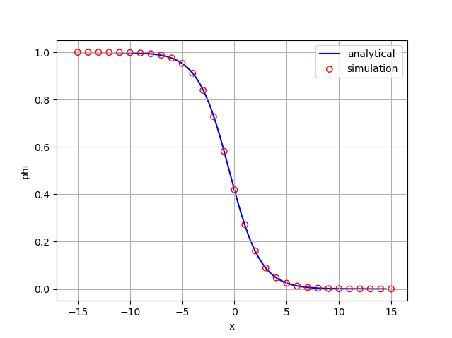
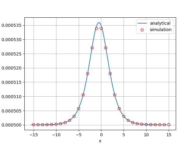
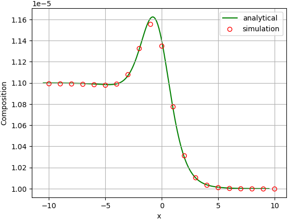
Those analytical solutions can be run in folders Analytical_Profile1 and Analytical_Profile2 of directory TestCase19_Surfactant. The post-processing used version 5.12 of paraview.

Examples of simulations with that model

Rising bubble and falling droplet

Rayleigh-Taylor instability and droplets coalescence

Section author: Alain Cartalade