Model of Navier-Stokes/Conservative Allen-Cahn (CAC)/Composition

Introduction

Basic model

That model is one of the most popular model of two-phase flows with interface-capturing. It is composed of incompressible Navier-Stokes (NS) equations coupled with the Conservative Allen-Cahn (CAC) equation (or levelset equation). That model is applied for simulating many classical problems such as “rising bubbles”, splashing droplets”, “Rayleigh-Taylor instability”, etc. In LBM_Saclay, that model is implemented in the kernel NSAC_Comp where _Comp means Composition equation. The kernel NSAC_Comp is extensively used for two-phase test cases which are contained in the folder run_training_lbm. The test cases of this folder are used in a training session of LBM with the Training version of LBM_Saclay.

• Practice of two-phase flows with test cases of run_training_lbm with that model can be performed with .ini input files of folder run_training_lbm.

That model is a basis for other models which are developed in other kernels e.g. two-phase flows with surfactant, two-phase flows with phase change, two-phase flows interacting with a solid phase and three immiscible fluids:

• Model of Navier-Stokes/CAC with surfactant

• Model of Navier-Stokes/CAC with Liquid-Gas phase change

• Model of Navier-Stokes/Allen-Cahn/Composition interacting with a solid phase

• Model of fluid flow for three immiscible phases

Mathematical model of incompressible two-phase flows

The mathematical model is composed of incompressible Navier-Stokes equations coupled with the phase-field equation and the composition equation.

Mathematical model

Mass balance equation

The mass balance writes:

(31)\[\boldsymbol{\nabla}\cdot\boldsymbol{u}=0\]

where \(\boldsymbol{u}\equiv\boldsymbol{u}(\boldsymbol{x},t)=(u_x,u_y,u_z)^T\) is the fluid velocity.

Impulsion balance equation

The impulsion balance equation writes:

(32)\[\varrho(\phi,c)\left[\frac{\partial\boldsymbol{u}}{\partial t}+\boldsymbol{\nabla}\cdot(\boldsymbol{u}\boldsymbol{u})\right]=-\boldsymbol{\nabla}p_{h}+\boldsymbol{\nabla}\cdot\left[\eta(\phi)\left(\boldsymbol{\nabla}\boldsymbol{u}+\boldsymbol{\nabla}\boldsymbol{u}^{T}\right)\right]+\boldsymbol{F}_{tot}\]

where \(p_{h}\equiv p_{h}(\boldsymbol{x},t)\) is the hydrodynamic pressure, \(\varrho\) is the total densiy and \(\eta\) is the dynamic viscosity. Those quantities are obtained from the interpolation of bulk properties with the phase-field \(\phi\). Their expressions will be given in the subsection “Closure”.

Phase-field equation

The interface is followed by an additional PDE on the phase-field:

(33)\[\frac{\partial\phi}{\partial t}+\boldsymbol{\nabla}\cdot(\boldsymbol{u}\phi)=\boldsymbol{\nabla}\cdot\left[M_{\phi}\left(\boldsymbol{\nabla}\phi-\frac{4}{W}\phi(1-\phi)\boldsymbol{n}\right)\right]+\lambda\mathscr{S}_{\phi}\]

where \(\phi\equiv\phi(\boldsymbol{x},t)\) is the phase-field, \(M_{\phi}\) is the mobility and \(W\) is the interface width. That equation is called “Conservative Allen-Cahn” equation (CAC). It is also encountered in the literature as the “Levelset” equation.

Composition equation

Finally, the composition equation is also considered in that model:

(34)\[\frac{\partial c}{\partial t}+\boldsymbol{\nabla}\cdot(\boldsymbol{u}c)=\boldsymbol{\nabla}\cdot\left[\mathcal{D}(\phi)\boldsymbol{\nabla}\mu_{c}\right]\]

where \(c\equiv c(\boldsymbol{x},t)\) is the composition, \(\mathcal{D}(\phi)\) is the diffusion coefficient and \(\mu_{c}\) is the chemical potential relative to the composition \(c\).

Force and source terms

Total force

Several forces are defined in NSAC_Comp kernel.

Total force

The total force \(\boldsymbol{F}_{tot}\) in Eq. (333) is defined by

(35)\[\boldsymbol{F}_{tot}=\boldsymbol{F}_{c}+\boldsymbol{F}_{g}+\boldsymbol{F}_{M}\]

where \(\boldsymbol{F}_{c}\) is the capillary force, \(\boldsymbol{F}_{g}\) is the gravity force and \(\boldsymbol{F}_{M}\) is the Marangoni force.

Gravity force

The gravity force \(\boldsymbol{F}_{g}\) is defined by

(36)\[\boldsymbol{F}_{g}=\varrho(\phi,c)\boldsymbol{g}\]

where \(\varrho(\phi,c)\) is an interpolation of bulk densities by Eq. (66)

Capillary force

The capillary force \(\boldsymbol{F}_{c}\) is defined by

(37)\[\boldsymbol{F}_{c}=\mu_{\phi}\boldsymbol{\nabla}\phi\]

where the chemical potential \(\mu_{\phi}\) is defined by

(38)\[\mu_{\phi}=\frac{3}{2}\sigma\left[\frac{16}{W}\phi(1-\phi)(1-2\phi)-W\boldsymbol{\nabla}^{2}\phi\right]\]

\(\sigma\) is the surface tension and \(W\) is the interface width.

Marangoni force

The Marangoni force \(\boldsymbol{F}_{M}\) is a surfacic gradient of \(\sigma(c)\) defined by

(39)\[\boldsymbol{F}_{M}=\frac{3W}{2}\left[\boldsymbol{\nabla}\sigma|\boldsymbol{\nabla}\phi|^{2}-\boldsymbol{\nabla}\phi(\boldsymbol{\nabla}\phi\cdot\boldsymbol{\nabla}\sigma)\right]\]

(40)\[\sigma(c)=\sigma_{ref}+\frac{d\sigma}{dc}(c-c_{ref})\]

(41)\[\frac{d\sigma}{dc}=\sigma_{c}<0\]

Source term of Eq. (33)

In the last term of the right-hand side of Eq. (33), the source term \(\mathscr{S}_{\phi}\) can be defined for phase-change problems. An example of such a source term can be found on Model of dissolution (Eq. (103)) and Model of crystal growth. In that case, the \(\lambda\) coefficient must be appropriately chosen. For two immiscible fluid flows, that coefficient is set equal to zero.

Closure relationships

Closure relationships

In order to close the model, it is required to add closure relationships. In Eq. (34), the flux is given by the gradient of chemical potential \(\mu_c\) which is generalization of the classic Fick’s law. The chemical potential is related to the composition \(c\) by

(42)\[\mu_{c}=\mu_{c}^{eq}+c(\phi,\mu_{c})-\left[c_{1}^{eq}\phi+c_{0}^{eq}(1-\phi)\right]\]

In that equation, \(\mu_{c}^{eq}\), \(c_{0}^{eq}\) and \(c_{1}^{eq}\) are three scalar values which must be set in the input file. If all of them are zero, then the classic diffusion equation is recoved. Non-zero positive values of \(c_{0}^{eq}\) and \(c_{1}^{eq}\) mean that the compositions in each phase will tend to the equilibrium compositions \(c_{0}^{eq}\) and \(c_{1}^{eq}\) during the simulation.

The total density \(\varrho\) is interpolated by \(\phi\) and \(c\):

(43)\[\varrho(\phi,c)=\rho_{1}(c)p(\phi)+\rho_{0}(c)(1-p(\phi))\]

In NSAC_Comp the bulk density can slightly vary with the composition. The interpolation is linear in \(c\) between the initial density \(\rho^{ini}\) and the equilibrium one \(\rho^{eq}\):

(44)\[\rho_{\Phi}(c)=(\rho_{\Phi}^{eq}-\rho_{\Phi}^{ini})\frac{c-c_{\Phi}^{ini}}{c_{\Phi}^{eq}-c_{\Phi}^{ini}}+\rho_{\Phi}^{ini}\]

It is recommended to keep the variation of \(\Delta \rho = \rho^{ini}-\rho^{eq}\) small. The index \(\Phi=0,1\) indicates phase 0 or phase 1. The interpolation function \(p(\phi)\) can be chosen:

(45)\[\begin{split}p(\phi)=\begin{cases} \phi\qquad\text{or}\\ \phi^{2}(3-2\phi) \end{cases}\end{split}\]

The dynamic viscosity is interpolated by a harmonic mean formula:

(46)\[\frac{1}{\eta(\phi)}=\frac{\phi}{\eta_{1}}+\frac{1-\phi}{\eta_{0}}\]

Finally in the composition equation, the diffusion parameter is also linearly interpolated:

(47)\[\mathcal{D}(\phi)=D_{1}\phi+D_{0}(1-\phi)\]

Alternative phase-field model

Alternative phase-field model

With the kernel NSAC_Comp, other phase-field equations can be simulated with appropriate options inside the input file. For example, the well-known model of Cahn-Hilliard writes:

Cahn-Hilliard model

(48)\[\frac{\partial\phi}{\partial t}+\boldsymbol{\nabla}\cdot(\boldsymbol{u}\phi)=\mathcal{M}_{\phi}\boldsymbol{\nabla}^{2}\mu_{\phi}\]

where the chemical potential is defined by

(49)\[\mu_{\phi}=2H\phi(1-\phi)(1-2\phi)-\zeta\boldsymbol{\nabla}^{2}\phi\]

Alternative form of conservative Allen-Cahn equation

The counter term \((4/W)\phi(1-\phi)\boldsymbol{n}\) in the Conservative Allen-Cahn (CAC) Eq. (33) can also be put outside the divergence term and noted \(\mathcal{S}_{ct}\):

(50)\[\frac{\partial\phi}{\partial t}+\boldsymbol{\nabla}\cdot(\boldsymbol{u}\phi)=M_{\phi}\boldsymbol{\nabla}^{2}\phi\underbrace{-\boldsymbol{\nabla}\cdot\left[\frac{4}{W}\phi(1-\phi)\boldsymbol{n}\right]}_{\mathcal{S}_{ct}}\]

Allen-Cahn equation for phase change problems

For problems of phase change, e.g. dissolution of porous media, the phase-field equation makes appear a first term involving the derivative of double-well \(\mathcal{S}_{dw}\) and a second term, a source term, \(\mathcal{S}_{st}\) which is responsible for the interface displacement and proportional to a coupling coefficient \(\lambda\). Such a model is presented in Model of dissolution where the phase-field equation writes:

(51)\[\frac{\partial\phi}{\partial t}+\boldsymbol{\nabla}\cdot(\boldsymbol{u}\phi)=M_{\phi}\boldsymbol{\nabla}^{2}\phi\underbrace{-\frac{M_{\phi}}{W^{2}}2\phi(1-\phi)(1-2\phi)}_{\mathcal{S}_{dw}}+\underbrace{\frac{\lambda M_{\phi}}{W^{2}}\mathscr{S}_{\phi}(\phi,\,\overline{\mu})}_{\mathcal{S}_{st}}\]

General form of phase-field equation

General formulation for phase-field equation

Finally, if we introduce two integers \(\chi_1\) and \(\chi_2\), a general formulation of the phase-field equation writes:

(52)\[\frac{\partial\phi}{\partial t}+\boldsymbol{\nabla}\cdot(\boldsymbol{u}\phi)=M_{\phi}\boldsymbol{\nabla}^{2}[\chi_{1}\mu_{\phi}+(1-\chi_{1})\phi]-(1-\chi_{1})\left[\chi_{2}\mathcal{S}_{ct}+(1-\chi_{2})\mathcal{S}_{dw}+\mathcal{S}_{st}\right]\]

In that equation if

• \(\chi_1=1\) then the CH Eq. (48) is recovered.

• \(\chi_1=0\) and \(\chi_2=1\), then the CAC Eq. (33) is recovered.

• \(\chi_1=0\) and \(\chi_2=0\), then the CAC Eq. (51) is recovered.

In the input file of LBM_Saclay, the integers \(\chi_1\) and \(\chi_2\) are respectively named cahn_hilliard and counter_term. Examples of .ini input files are given in the folder run_training_lbm

• For Cahn-Hilliard model: TestCase05_Spinodal-Decomposition2D

• For Allen-Cahn equation with phase change: TestCase06b_Stefan-Problem

• For Conservative Allen-Cahn equation: all other two-phase test cases (e.g. TestCase09_Capillary-Wave2D)

List of input parameters in .ini file

Section [lbm]

In section [lbm] use the keyword problem=NSAC_Comp to simulate that mathematical model. Next, the sections [params] and [params_composition] must be set.

[params]

The list of parameters are summarized in Table below.

Math symbol	Parameter name	Equation	.ini file
\(M_{\phi}\)	Mobility of interface	Eq. (33)	Mphi
\(W\)	Interface width	Eq. (33)	W
\(\lambda\)	Coupling parameter	Eq. (33)	lambda
\(\rho_0\)	Bulk density of phase 0	Eq. (143)	rho0
\(\rho_1\)	Bulk density of phase 1	Eq. (143)	rho1
\(\nu_0\)	Kinematic viscosity of phase 0	Eq. (144)	nu0
\(\nu_1\)	Kinematic viscosity of phase 1	Eq. (144)	nu1
\(\sigma\)	Surface tension	Eq. (82)	sigma
\(g_{\alpha}\) with \(\alpha=x,y,z\)	Gravity	Impulsion balance	gy
\(D_0\)	Bulk diffusion of phase 0	Eq. (47)	rho0
\(D_1\)	Bulk diffusion of phase 1	Eq. (47)	rho1
\(\rho_{0}^{ini}\)	Initial bulk density of phase 0	Eq. (44)	rho0
\(\rho_{0}^{eq}\)	Equilibrium bulk density of phase 0	Eq. (44)	rho1
\(\rho_{1}^{ini}\)	Initial bulk density of phase 0	Eq. (44)	rho0
\(\rho_{1}^{eq}\)	Equilibrium bulk density of phase 0	Eq. (44)	rho1

[params_composition]

Math symbol	Parameter name	Equation	.ini file
\(\mu^{eq}_c\)	Equilibrium chemical potential	Eq. (42)	mu_eq
\(c_0^{ini}\)	Initial composition of phase 0	Init cond for Eq. (34)	c0_inf
\(c_0^{eq}\)	Equilibrium composition of phase 0	Eq. (42)	c0_co
\(c_1^{ini}\)	Initial composition of phase 1	Init cond for Eq. (34)	c1_inf
\(c_1^{eq}\)	Equilibrium composition of phase 1	Eq. (42)	c1_co

[params_marangoni]

• force_marangoni=: 1 or 0

• sigma_marangoni=: positive real value (Eq. (40))

• dsigmadcomp =: negative real value (Eq. (41))

[output]

In the output section [output] of .ini file, the fields to write must be indicated as a list in write_variables=. For example:

write_variables=vx,vy,vz,pressure,phi,composition

The names of fields can be found in the source file Index_NS_AC_Comp.h of directory LBM_Saclay_Rech-Dev/src/kernels/NSAC_Comp.

Validation with analytical solution of Prosperetti

That analytical solution has been implemented in sage math (see ref [2])

Results

Mesh 128x256

For that first simulation the mesh is composed of 128x256 cells corresponding to \(\delta x=1\). We also set \(\delta t=1\). The total number of time-steps is set equal to \(N_t=300001\) (nStepmax) and nOutput=2000. The simulation took 222.9 seconds (~3min43s). The comparison is presented on Fig. Fig. 31.

Mesh 256x512

For that first simulation the mesh is composed of 256x512 cells corresponding to \(\delta x=0.5\). We also set \(\delta t=0.5\). The total number of time-steps is set equal to \(N_t=600001\) (nStepmax) and nOutput=4000. The simulation took 1042.3 seconds (~17min22s). The comparison is presented on Fig. Fig. 32.

2085.389 s.

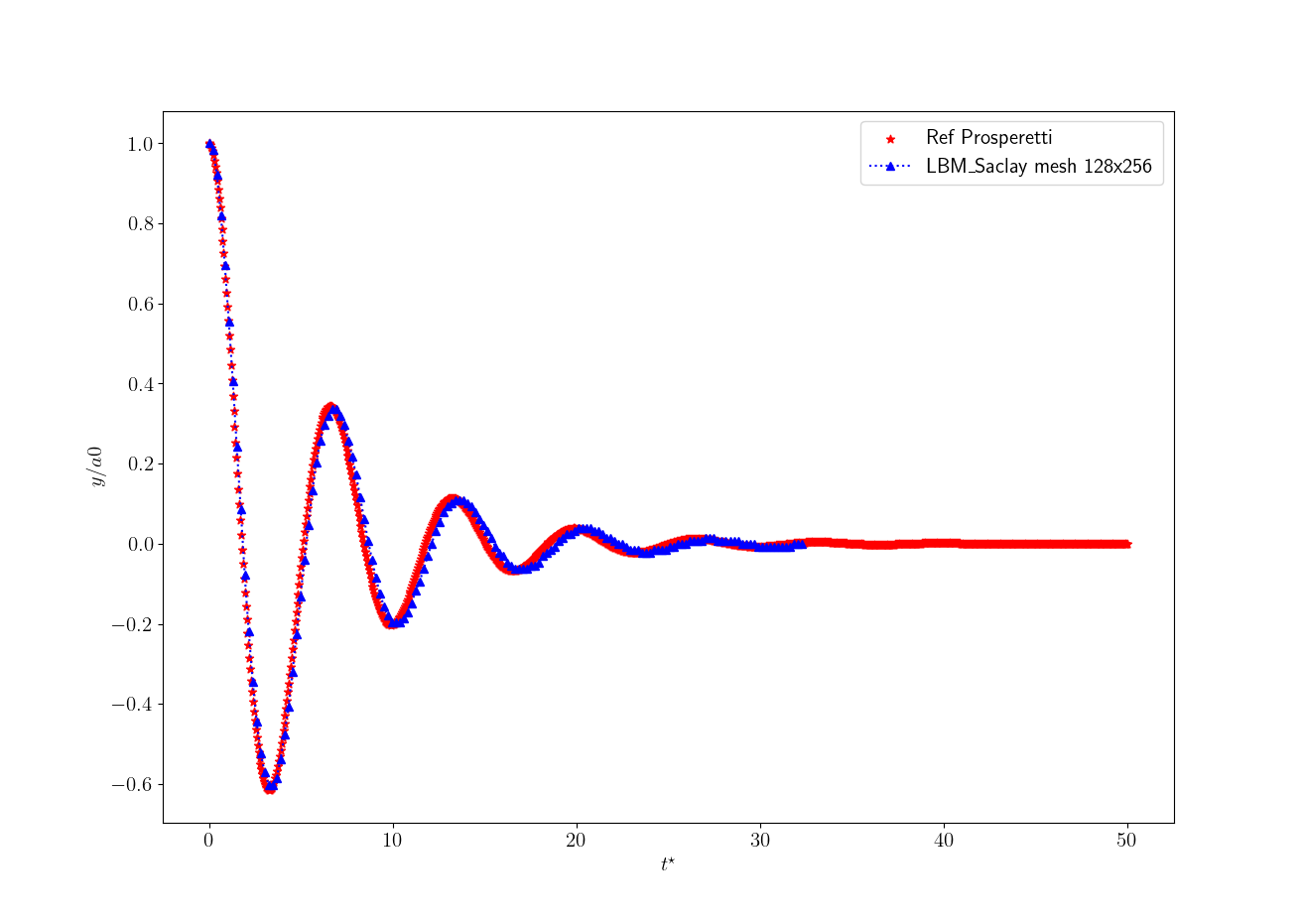
Fig. 31 Comparison on mesh size 128x256 and \(\delta x=\delta t=1\).

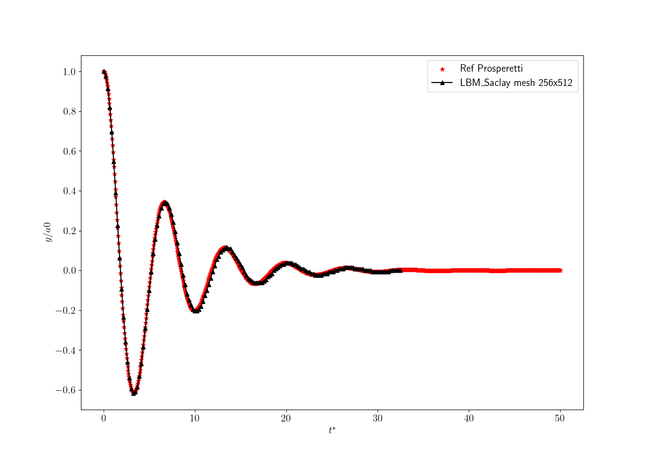
Fig. 32 Comparison on mesh size 256x512 and \(\delta x=\delta t=0.5\).

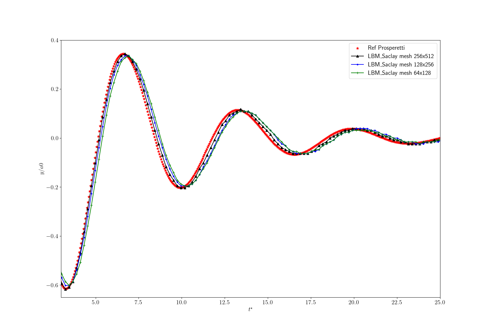
Fig. 33 Zoom for mesh sizes 64x128 (green), 128x256 (blue) and 256x512 (black) with reference (red).

As expected, the numerical solution becomes more and more accurate when the mesh size and time step diminish.

Setup for LBM_Saclay

The simulations with LBM_Saclay are run with kernel NSAC_Comp. Even though the composition equation is solved in that kernel, the composition is not used for that test case. The collision operators are BGK for phase-field and composition equations. For Navier-Stokes equations, the MRT is used.

Input parameters

In .ini files, the following parameters are identical:

• For hydrodynamic the parameters are \(\rho_l=1\), \(\rho_g=0.01\), \(\nu_l=\nu_g=0.005\), \(g_y=0\), \(\sigma=10^{-4}\).

• For phase-field equation, they are \(W=5\), \(M_{\phi}=0.02\).

The positions of boundaries are

• \(x_{min}=-64\), \(x_{max}=64\) corresponding to \(L_x=128\). The conditions are periodic.

• \(y_{min}=0\), \(y_{max}=256\) corresponding to \(L_y=256\). The conditions are bounce-back.

For following simulations \(L_x=128\) and \(L_y=256\) are set constant. We modify \(N_x\) and \(N_y\) i.e. \(\delta x\) and \(\delta t\). For those comparisons, the density ratio is \(\rho_l/\rho_g=100\). For higher density ratios (~830) the comparisons are presented in Run “Two-phase with fluid flows”. The simulations ran on MANWE equipped with one GPU A6000.

• The wavelength is \(\lambda=L_x\) and the initial amplitude \(a_0\) is set equal to \(L_x/100=1.28\)

Examples of simulations with that model

As already mentioned, many test cases using that math model can be found in the directory run_training_lbm to Practice of two-phase flows with test cases of run_training_lbm. It is recommended to start running the .ini files contained in that directory. Here we present few videos of 3D simulations. Other videos can be found in Run “Two-phase with fluid flows”

Bibliography

[1]

Andrea Prosperetti. Motion of two superposed viscous fluids. The Physics of Fluids, 24(7):1217–1223, 07 1981. URL: https://doi.org/10.1063/1.863522.

[2]

Hoel Keraudren. Pseudo-potential method for multiphase flows using Lattice Boltzmann Methods (Simulation of Navier-Stokes-Korteweg equations). Technical Report CEA, 2023.

Section author: Alain Cartalade