Model of solidification and crystal growth

Useful thermodynamic relations for phase change

Specific heat (dim \([\text{E}]/([\text{M}].[\Theta])\)

At constant pressure

(578)\[C_{P}\,\hat{=}\,T\left(\frac{\partial s}{\partial T}\right)_{P}\]

At constant volume

(579)\[C_{v}\,\hat{=}\,T\left(\frac{\partial s}{\partial T}\right)_{\rho}\]

Latent heat at melting temperature \(T_m\) (dim [E]/[M])

(580)\[\mathcal{L}\,\hat{=}\,T_m(s_{l}(T_m)-s_{s}(T_m))\]

Thermodynamic Maxwell relations

(581)\[\left(\frac{\partial T}{\partial v}\right)_{s}=-\left(\frac{\partial P}{\partial s}\right)_{v}\]

(582)\[-\left(\frac{\partial s}{\partial P}\right)_{T}=\left(\frac{\partial v}{\partial T}\right)_{P}\]

(583)\[-\left(\frac{\partial s}{\partial v}\right)_{T}=-\left(\frac{\partial P}{\partial T}\right)_{v}\]

(584)\[\left(\frac{\partial T}{\partial P}\right)_{s}=-\left(\frac{\partial v}{\partial s}\right)_{P}\]

Proof of Eq. (581) with \(\mathcal{U}(V,S)\)

\[\begin{split}\frac{\partial\mathcal{U}}{\partial V\partial S}=\frac{\partial\mathcal{U}}{\partial S\partial V}&\Longleftrightarrow\frac{\partial}{\partial V}\underbrace{\left(\frac{\partial\mathcal{U}}{\partial S}\right)}_{\equiv T}=\frac{\partial}{\partial S}\underbrace{\left(\frac{\partial\mathcal{U}}{\partial V}\right)}_{\equiv-P}\\ &\Longleftrightarrow\left(\frac{\partial T}{\partial V}\right)_{S}=-\left(\frac{\partial P}{\partial S}\right)_{V}\end{split}\]

Proof of Eq. (583) with \(\mathcal{F}(V,T)\)

\[\begin{split}\frac{\partial\mathcal{F}}{\partial V\partial T}=\frac{\partial\mathcal{F}}{\partial T\partial V}&\Longleftrightarrow\frac{\partial}{\partial V}\underbrace{\left(\frac{\partial\mathcal{F}}{\partial T}\right)}_{\equiv-S}=\frac{\partial}{\partial T}\underbrace{\left(\frac{\partial\mathcal{F}}{\partial V}\right)}_{\equiv-P}\\ &\Longleftrightarrow-\left(\frac{\partial S}{\partial V}\right)_{T}=-\left(\frac{\partial P}{\partial T}\right)_{V}\end{split}\]

Solidification of a pure substance and Stefan’s problem

We consider at the melting temperature \(T_m\), the coexistence of a chemical specie \(A\) into two phases: a tiny solid seed inside a liquid bath of same specie. The temperature of the system \(T\) is quenched below the melting temperature \(T<T_m\). Then the solidification occurs: the small seed grows i.e. the liquid becomes solid and the excess of latent heat \(\mathcal{L}\) is released at the interface and advected with the normal velocity of the interface \(v_n\). The modeling of that phase change problem is performed with the classical Stefan’s problem.

Stefan’s problem of phase change

The Stefan’s model of phase change is composed of three equations: the heat equation with two conditions at interface between solid and liquid:

(585)\[C_{p}\frac{\partial T}{\partial t}=\Lambda_{\Phi}\boldsymbol{\nabla}^{2}T\]

where \(T\) is the temperature, \(\Lambda_{\Phi}\) is the thermal conductivity for both phases \(\Phi=0,1\). The first interface condition is the Stefan condition (conservation at interface):

(586)\[\mathcal{L}v_{n}=(C_{p}\Lambda\boldsymbol{\nabla}T|_{sol}-C_{p}\Lambda\boldsymbol{\nabla}T|_{liq})\cdot\hat{\boldsymbol{n}}\]

where \(\hat{\boldsymbol{n}}\) is the normal vector at interface, and \(v_{n}\) the normal velocity of the interface, \(\mathcal{L}\) is the latent heat. The second interface condition is the Gibbs-Thomson condition:

(587)\[T_{i}=T_{m}-\frac{\sigma T_{m}}{\mathcal{L}}\kappa-\frac{v_{n}}{m_{k}}\]

where \(T_i\) is the temperature at the interface, \(T_{m}\) is the melting temperature, \(\sigma\) is the surface tension, \(\mathcal{L}\) is the latent heat, \(\kappa\) is the curvature, \(m_{k}\) is the interface mobility, and \(v_{n}\) is the normal velocity of interface.

Derivation of phase-field model

The derivation of the phase-field model of solidification is inspired from [1]. For derivation of crystal growth model see [2] and [3].

Free energy density \(\mathscr{F}\)

The Stefan’s problem is a “sharp interface” modelling. Here, an equivalent diffuse interface is derived. We introduce a phase-field \(\psi(\boldsymbol{x},t)\) with \(\psi=-1\) in the solid phase and \(\psi=+1\) in the liquid phase. The solid (respectively liquid) is characterized by its specific heat \(C_p^s\) (resp. \(C_p^l\)) and thermal conductivity \(\Lambda^s\) (resp. \(\Lambda^s\)). The interface is characterized by its normal velocity \(v_n\), the unit normal vector \(\boldsymbol{n}_{\psi}\) and the latent heat \(\mathcal{L}\). The solidification problem is presented on Fig. Fig. 63

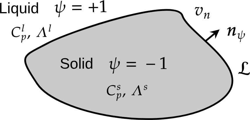
Fig. 63 Solidification

Functional of free energy

Functional of free energy

The free energy density is now the functional of two functions \(\psi\) and \(T\)

(588)\[\mathscr{F}[\psi,{\color{red}T}]=\int\Bigl[\underbrace{\mathcal{F}_{int}(\psi,\boldsymbol{\nabla}\psi)}_{\text{Standard interface free energy}}+\underbrace{{\color{red}f_{bulk}(\psi,T)}}_{\text{Thermodynamic of bulks}}\Bigr]dV\]

That free energy density contains two contributions: the first one is the interface contribution \(\mathcal{F}_{int}(\psi,\boldsymbol{\nabla}\psi)\) and the second one the bulk free energy density \(f_{bulk}(\psi,T)\).

Interface contribution

The first one is standard and has been widely discussed until now. It is defined by a double-well plus a gradient energy term:

\[\mathcal{F}_{int}(\psi,\boldsymbol{\nabla}\psi)=f_{dw}(\psi)+\frac{\zeta}{2}(\boldsymbol{\nabla}\psi)^{2}\]

where the double-well is defined by

\[\begin{split}f_{dw}(\psi)&=Hg_{3}(\psi)\\ &=H(\psi-\psi^{\star})^{2}(\psi+\psi^{\star})^{2}\end{split}\]

the minima are \(\psi^{\star}=\pm1\). With that double-well free energy, the Euler-Lagrange solution and the interface have already been discussed in Alternative forms of double-wells: the equilibrium solution is \(\psi^{eq}(x)=\psi^{\star}\tanh\left(2x/W\right)\), the interface width is \(W=\frac{1}{\psi^{\star}}\sqrt{\frac{2\zeta}{H}}\) and the surface tension is \(\sigma=\frac{4}{3}\sqrt{2\zeta H}\).

Bulk contribution

The bulk free energy density takes into account the free energy of each phase \({\color{red}f_{s}(T)}\) in the solid and \({\color{red}f_{l}(T)}\) in the liquid:

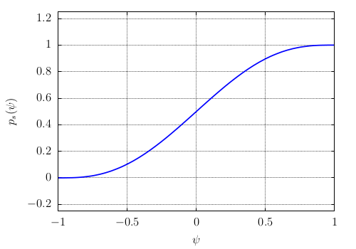
(589)\[f_{bulk}(\psi,T)=p_{s}(\psi){\color{red}f_{s}(T)}+\left[1-p_{s}(\psi)\right]{\color{red}f_{l}(T)}\]

where \(p_{s}(\psi)\) is an interpolation polynomial defined by:

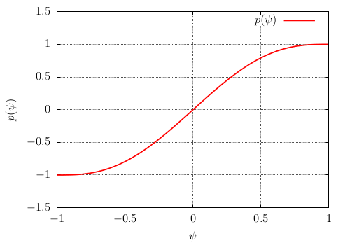
(590)\[p_{s}(\psi)=\frac{1+p(\psi)}{2}\]

of minimum and maximum values between 0 and 1 (see Fig. Fig. 64). It is defined by \(p(\psi)\) of minimum and maximum values -1 and +1 (see Fig. Fig. 65)

(591)\[p(\psi)=\frac{15}{8}\left[\psi-\frac{2}{3}\psi^{3}+\frac{\psi^{5}}{5}\right]\]

Fig. 64 Interpolation function \(p_s(\psi)\)

Fig. 65 Interpolation function \(p(\psi)\)

Variation of \(\mathscr{F}\)

The variation of \(\mathscr{F}\) writes:

(592)\[\delta\mathscr{F}=\int\left\{ -\zeta\boldsymbol{\nabla}^{2}\psi+f_{dw}^{\prime}(\psi)+\frac{p^{\prime}(\psi)}{2}\left[f_{s}(T)-f_{l}(T)\right]\right\} \delta\psi+\left\{ p_{s}(\psi)\frac{\partial f_{s}(T)}{\partial T}+[1-p_{s}(\psi)]\frac{\partial f_{l}(T)}{\partial T}\right\} \delta TdV\]

Temperature equation

Temperature equation

The conservation of internal energy density \(e\) writes:

(593)\[\frac{\partial e}{\partial t}=\boldsymbol{\nabla}\cdot(\Lambda\boldsymbol{\nabla}T)\]

where the Fourier law has been assumed for the diffusive flux. After expressing the internal energy \(e(\phi,s)\) as a function of \(T\) (see proof below), we obtain:

(594)\[\boxed{C_{p}\frac{\partial T}{\partial t}=\boldsymbol{\nabla}\cdot(\Lambda\boldsymbol{\nabla}T)-\underbrace{\frac{1}{2}p^{\prime}(\psi)\mathcal{L}\frac{\partial\psi}{\partial t}}_{\text{Latent heat at interface}}}\]

Proof

• Variation of \(\mathscr{F}\) wrt \(T\): opposite of entropy

  (595)\[\begin{split}s(\psi,T)&=-\frac{\delta\mathscr{F}}{\delta T}\\ &=-\frac{\partial f_{bulk}(\psi,T)}{\partial T}\\ &=-p_{s}(\psi)\underbrace{\frac{\partial f_{s}}{\partial T}}_{s_{s}(T)}-\left[1-p_{s}(\psi)\right]\underbrace{\frac{\partial f_{l}}{\partial T}}_{s_{l}(T)}\end{split}\]

• Thermo identity (\(de=Tds\)) and chain rule

  \[\begin{split}de&=Tds(\psi,T)\\ &=\underbrace{T\frac{\partial s}{\partial T}}_{C_{p}\text{: specific heat}}dT+T\underbrace{\frac{\partial s}{\partial\psi}}_{\text{use previous Eq.}}d\psi\end{split}\]

  For the first term of the right-hand side we use the definition of specific heat Eq. (). For the second term we derive Eq. () wrt \(\psi\). After division by \(dt\), we obtain

  (596)\[\frac{\partial e}{\partial t} =C_{p}\frac{\partial T}{\partial t}+p_{s}^{\prime}(\psi)\underbrace{T\left[s_{l}(T)-s_{s}(T)\right]}_{\equiv\mathcal{L}\text{: latent heat}}\frac{\partial\psi}{\partial t}\]

  Finally by replacing Eq. () in Eq. (), we obtain Eq. ().

Phase-field equation

The dynamic of \(\psi\) must obey to the following Allen-Cahn equation Eq. (452) to minimize the free energy:

(597)\[\frac{1}{\mathscr{M}_{\psi}}\frac{\partial\psi}{\partial t}=-\frac{\delta\mathscr{F}}{\delta\psi}\]

To calculate the variation of \(\mathscr{F}\) wrt \(\psi\), we use Eq. ():

\[\begin{split}\frac{1}{\mathscr{M}_{\psi}}\frac{\partial\psi}{\partial t}&={\color{gray}-\frac{\delta\mathscr{F}_{int}(\psi,\boldsymbol{\nabla}\psi)}{\delta\psi}}-\frac{\partial f_{bulk}(\psi,T)}{\partial\psi}\\ &={\color{gray}\zeta\boldsymbol{\nabla}^{2}\psi-f_{dw}^{\prime}(\psi)}-\underbrace{\frac{p^{\prime}(\psi)}{2}\left[f_{s}(T)-f_{l}(T)\right]}_{\text{Thermodynamic driving source}}\end{split}\]

To simplify the thermodynamic driving source, a common hypothesis is to consider the temperature \(T\) close to the melting temperature \(T_m\). A Taylor expansion yields:

(598)\[f_{\Phi}(T)\sim f_{\Phi}(T_{m})+\left.\frac{\partial f_{\Phi}}{\partial T}\right|_{T_{m}}(T-T_{m})\]

where \(\Phi=s,l\). At \(T_m\), \(f_l(T_m)=f_s(T_m)\) and the latent heat is () \(\mathcal{L}=T_{m}[s_{l}(T_{m})-s_{s}(T_{m})]\). Finally

\[\frac{1}{\mathscr{M}_{\psi}}\frac{\partial\psi}{\partial t}=\zeta\boldsymbol{\nabla}^{2}\psi-Hg_{3}^{\prime}(\psi)-\frac{p^{\prime}(\psi)}{2}\frac{\mathcal{L}}{T_{m}}(T-T_{m})\]

In the right-hand side, the coefficient \(H\) is set in factor:

(599)\[\frac{1}{\mathscr{M}_{𝜓}}\frac{\partial\psi}{\partial t}=H\left[\frac{\zeta}{H}\boldsymbol{\nabla}^{2}𝜓-g_{3}^{\prime}(𝜓)-\frac{1}{H}\frac{p^{\prime}(𝜓)}{2}\frac{\mathcal{L}}{T_{m}}(T-T_{m})\right]\]

and we define new coefficients:

Characteristic time

(600)\[\tau_{0}=\frac{1}{(H\mathscr{M}_{\psi})}\]

Interface width

(601)\[W_{0}=\sqrt{\frac{\zeta}{H}}\]

Coupling coefficient

(602)\[\lambda=\frac{1}{H}\]

Finally, using Eqs. (600), (601) and (602) in Eq. (599) we obtain for the phase-field equation:

Phase-field equation

(603)\[\tau_{0}\frac{\partial𝜓}{\partial t}=W_{0}^{2}\boldsymbol{\nabla}^{2}𝜓-g_{3}^{\prime}(𝜓)-\lambda\frac{p^{\prime}(𝜓)}{2}\frac{\mathcal{L}}{T_{m}}(T-T_{m})\]

Summary

Phase-field model of solidification

The phase-field model of solidification is composed of one phase-field equation for the interface:

(604)\[\tau_{0}\frac{\partial𝜓}{\partial t}=W_{0}^{2}\boldsymbol{\nabla}^{2}𝜓-g_{3}^{\prime}(𝜓)-\lambda\frac{p^{\prime}(𝜓)}{2}\frac{\mathcal{L}}{T_{m}}(T-T_{m})\]

coupled with one temperature equation:

(605)\[C_{p}\frac{\partial T}{\partial t}=\boldsymbol{\nabla}\cdot(\Lambda\boldsymbol{\nabla}T)-\underbrace{\frac{1}{2}p^{\prime}(\psi)\mathcal{L}\frac{\partial\psi}{\partial t}}_{\text{Latent heat at interface}}\]

Equivalence between phase-field model and Stefan’s problem

Equivalence between sharp and diffuse interface models

The sharp interface model (Stefan’s problem) and the phase-field model expressed with the dimensionless temperature \(\theta=(T-T_{m})C_{p}/\mathcal{L}\) write:

Stefan’s problem with dimnesionless temperature

\[\begin{split}\frac{\partial\theta}{\partial t}&=D\boldsymbol{\nabla}^{2}\theta\\ v_{n}&=D\hat{\boldsymbol{n}}\cdot(\boldsymbol{\nabla}\theta|_{sol}-\boldsymbol{\nabla}\theta|_{liq})\\ \theta_{i}&=-{\color{red}d_{0}}\kappa-{\color{red}\beta}v_{n}\end{split}\]

Phase-field model with dimensionless temperature

\[\begin{split}\frac{\partial\theta}{\partial t}&=D\boldsymbol{\nabla}^{2}\theta-\frac{1}{2}p^{\prime}(\psi)\frac{\partial\psi}{\partial t}\\ {\color{blue}\tau_{0}}\frac{\partial\psi}{\partial t}&={\color{blue}W_{0}^{2}}\boldsymbol{\nabla}^{2}\psi-g_{3}^{\prime}(\psi)-{\color{blue}\lambda}\frac{p^{\prime}(\psi)}{2}\theta\end{split}\]

where \(\theta\) is the dimensionless temperature, \(d_{0}=\sigma_{0}T_{m}C_{p}/\mathcal{L}^{2}\) is the capillary length, and \(\beta=C_{p}/\mathcal{L}m\) is the kinetic coefficient. With the matched asymptotic expansions, it is proved that both models are equivalent provided that the two following conditions hold:

(606)\[{\color{red}d_{0}}={\color{teal}a_{1}}\frac{{\color{blue}W_{0}}}{{\color{blue}\lambda}}\]

(607)\[{\color{red}\beta}={\color{teal}a_{1}}\left[\frac{{\color{blue}\tau_{0}}}{{\color{blue}\lambda}{\color{blue}W_{0}}}-{\color{teal}a_{2}}\frac{{\color{blue}W_{0}}}{D}\right]\]

where \({\color{teal}a_{1}}=0.8839\) and \({\color{teal}a_{2}}=0.6267\) (see [3]). In the right-hand side of Eqs. () and () \(\lambda\), \(W_{0}\) and \(\tau_{0}\) are the parameters of the phase-field model.

Anisotropy function and phase-field model of crystal growth

Dependence of properties with normal vector \(\boldsymbol{n}\equiv\boldsymbol{n}_{\psi}=-\boldsymbol{\nabla}\psi/\bigl|\boldsymbol{\nabla}\psi\bigr|\)

Surface tension \(\sigma\equiv\sigma(\boldsymbol{n})\)

(608)\[\sigma(\boldsymbol{n})=\sigma_{0}{\color{red}a_{s}(\boldsymbol{n})}\]

kinetic coefficient \(\beta\equiv\beta(\boldsymbol{n})\)

(609)\[\beta(\boldsymbol{n})=\beta_{0}{\color{red}a_{s}(\boldsymbol{n})}\]

Interface width \(W\equiv W(\boldsymbol{n})\)

(610)\[W(\boldsymbol{n})=W_{0}{\color{red}a_{s}(\boldsymbol{n})}\]

where the anisotropy function \(a_{s}(\boldsymbol{n})\) depends on the shape of crystal we want to simulate. Two anisotropy functions are presented below for main growing directions [100] and [110].

Definition of \(a_s(\boldsymbol{n})\) for [100] directions

(611)\[{\color{red}a_{s}(\boldsymbol{n})}=1+\epsilon_{s}\left[4(n_{x}^{4}+n_{y}^{4}+n_{z}^{4})-3\right]\]

where \(\epsilon_s\) is a positive parameter.

Fig. 66 Representation of Eq. (611)

Definition of \(a_s(\boldsymbol{n})\) for [110] directions

(612)\[a_{s}(\boldsymbol{n})=1+\epsilon_{s}\left(\sum_{\alpha}n_{\alpha}^{4}-\frac{3}{5}\right)+\delta\left(3\sum_{\alpha}n_{\alpha}^{4}+66n_{x}^{2}n_{y}^{2}n_{z}^{2}-\frac{17}{7}\right)\]

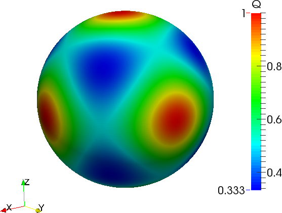
where \(\epsilon_s\) and \(\delta\) are positive parameters.

Fig. 67 Representation of Eq. (612)

Phase-field model of crystal growth

Phase-field equation

(613)\[\tau_{0}{\color{red}a_{s}^{2}(\boldsymbol{n})}\frac{\partial\psi}{\partial t}=W_{0}^{2}\boldsymbol{\nabla}\cdot\left[{\color{red}a_{s}^{2}(\boldsymbol{n})}\boldsymbol{\nabla}\psi\right]+\boldsymbol{\nabla}\cdot{\color{blue}\boldsymbol{\mathcal{N}}(\boldsymbol{n})}+\underbrace{(1-\psi^{2})\left[\psi-\lambda\theta(1-\psi^{2})\right]}_{\text{source term of phase change (0 in bulks)}}\]

where

(614)\[{\color{blue}\boldsymbol{\mathcal{N}}(\boldsymbol{n})}=W_{0}^{2}\bigl|\boldsymbol{\nabla}\psi\bigr|^{2}{\color{red}a_{s}(\boldsymbol{n})}\frac{\partial{\color{red}a_{s}(\boldsymbol{n})}}{\partial(\partial_{\alpha}\psi)}\]

and the anisotropy function \(a_s(\boldsymbol{n})\) is defined by Eq. (611).

Temperature equation

The temperature equation remains unchanged:

(615)\[\frac{\partial\theta}{\partial t}=D\boldsymbol{\nabla}^{2}\theta+\frac{1}{2}\frac{\partial\psi}{\partial t}\]

References

[1]

Mathis Plapp. Phase-Field Models, pages 129–175. Springer Vienna, 2012. doi:10.1007/978-3-7091-1227-4_4.

[2]

Alain Karma and Wouter-Jan Rappel. Phase-field method for computationally efficient modeling of solidification with arbitrary interface kinetics. Physical Review E, 53(4):R3017–R3020, 1996. doi:10.1103/PhysRevE.53.R3017.

[3] (1,2)

Alain Karma and Wouter-Jan Rappel. Quantitative phase-field modeling of dendritic growth in two and three dimensions. Phys. Rev. E, 57:4323–4349, Apr 1998. doi:10.1103/PhysRevE.57.4323.

Section author: Alain Cartalade