Model of solidification and crystal growth

Useful thermodynamic relations for phase change

Specific heat (dim \([\text{E}]/([\text{M}].[\Theta])\)

At constant pressure

(507)\[C_{P}\,\hat{=}\,T\left(\frac{\partial s}{\partial T}\right)_{P}\]

At constant volume

(508)\[C_{v}\,\hat{=}\,T\left(\frac{\partial s}{\partial T}\right)_{\rho}\]

Latent heat at melting temperature \(T_m\) (dim [E]/[M])

(509)\[\mathcal{L}\,\hat{=}\,T_m(s_{l}(T_m)-s_{s}(T_m))\]

Thermodynamic Maxwell relations

(510)\[\left(\frac{\partial T}{\partial v}\right)_{s}=-\left(\frac{\partial P}{\partial s}\right)_{v}\]

(511)\[-\left(\frac{\partial s}{\partial P}\right)_{T}=\left(\frac{\partial v}{\partial T}\right)_{P}\]

(512)\[-\left(\frac{\partial s}{\partial v}\right)_{T}=-\left(\frac{\partial P}{\partial T}\right)_{v}\]

(513)\[\left(\frac{\partial T}{\partial P}\right)_{s}=-\left(\frac{\partial v}{\partial s}\right)_{P}\]

Proof of Eq. () with \(\mathcal{U}(V,S)\)

\[\begin{split}\frac{\partial\mathcal{U}}{\partial V\partial S}=\frac{\partial\mathcal{U}}{\partial S\partial V}&\Longleftrightarrow\frac{\partial}{\partial V}\underbrace{\left(\frac{\partial\mathcal{U}}{\partial S}\right)}_{\equiv T}=\frac{\partial}{\partial S}\underbrace{\left(\frac{\partial\mathcal{U}}{\partial V}\right)}_{\equiv-P}\\ &\Longleftrightarrow\left(\frac{\partial T}{\partial V}\right)_{S}=-\left(\frac{\partial P}{\partial S}\right)_{V}\end{split}\]

Proof of Eq. () with \(\mathcal{F}(V,T)\)

\[\begin{split}\frac{\partial\mathcal{F}}{\partial V\partial T}=\frac{\partial\mathcal{F}}{\partial T\partial V}&\Longleftrightarrow\frac{\partial}{\partial V}\underbrace{\left(\frac{\partial\mathcal{F}}{\partial T}\right)}_{\equiv-S}=\frac{\partial}{\partial T}\underbrace{\left(\frac{\partial\mathcal{F}}{\partial V}\right)}_{\equiv-P}\\ &\Longleftrightarrow-\left(\frac{\partial S}{\partial V}\right)_{T}=-\left(\frac{\partial P}{\partial T}\right)_{V}\end{split}\]

Solidification of a pure substance and Stefan’s problem

We consider at the melting temperature \(T_m\), the coexistence of a chemical specie \(A\) into two phases: a tiny solid seed inside a liquid bath of same specie. The temperature of the system \(T\) is quenched below the melting temperature \(T<T_m\). Then the solidification occurs: the small seed grows i.e. the liquid becomes solid and the excess of latent heat \(\mathcal{L}\) is released at the interface and advected with the normal velocity of the interface \(v_n\). The modeling of that phase change problem is performed with the classical Stefan’s problem.

Stefan’s problem of phase change

The Stefan’s model of phase change is composed of three equations: the heat equation with two conditions at interface between solid and liquid:

(514)\[C_{p}\frac{\partial T}{\partial t}=\Lambda_{\Phi}\boldsymbol{\nabla}^{2}T\]

where \(T\) is the temperature, \(\Lambda_{\Phi}\) is the thermal conductivity for both phases \(\Phi=0,1\). The first interface condition is the Stefan condition (conservation at interface):

(515)\[\mathcal{L}v_{n}=(C_{p}\Lambda\boldsymbol{\nabla}T|_{sol}-C_{p}\Lambda\boldsymbol{\nabla}T|_{liq})\cdot\hat{\boldsymbol{n}}\]

where \(\hat{\boldsymbol{n}}\) is the normal vector at interface, and \(v_{n}\) the normal velocity of the interface, \(\mathcal{L}\) is the latent heat. The second interface condition is the Gibbs-Thomson condition:

(516)\[T_{i}=T_{m}-\frac{\sigma T_{m}}{\mathcal{L}}\kappa-\frac{v_{n}}{m_{k}}\]

where \(T_i\) is the temperature at the interface, \(T_{m}\) is the melting temperature, \(\sigma\) is the surface tension, \(\mathcal{L}\) is the latent heat, \(\kappa\) is the curvature, \(m_{k}\) is the interface mobility, and \(v_{n}\) is the normal velocity of interface.

Derivation of phase-field model

The derivation of the phase-field model of solidification is inspired from

Free energy density \(\mathscr{F}\)

The Stefan’s problem is a “sharp interface” modelling. Here, an equivalent diffuse interface is derived. We introduce a phase-field \(\psi=\pm1\): \(\psi=-1\) in the solid phase and \(\psi=+1\) in the liquid phase.

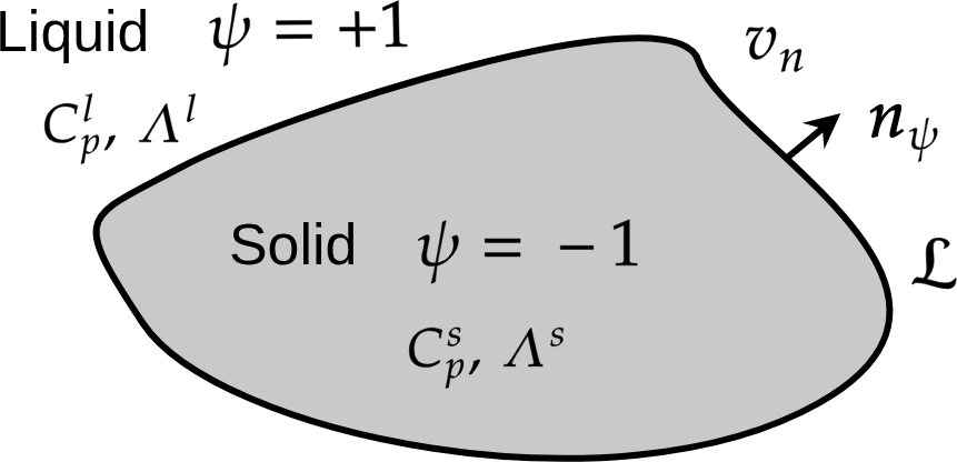
Fig. 54 Solidification

The free energy density is now the functional of two functions \(\psi\) and \(T\)

(517)\[\mathscr{F}[\psi,{\color{red}T}]=\int\Bigl[\underbrace{\mathcal{F}_{int}(\psi,\boldsymbol{\nabla}\psi)}_{\text{Standard interface free energy}}+\underbrace{{\color{red}f_{bulk}(\psi,T)}}_{\text{Thermodynamic of bulks}}\Bigr]dV\]

That free energy density contains two contributions: the first one is the interface contribution \(\mathcal{F}_{int}(\psi,\boldsymbol{\nabla}\psi)\) and the second one the bulk free energy density \(f_{bulk}(\psi,T)\). The first one is standard. It is defined by a double-well plus a gradient energy term:

\[\mathcal{F}_{int}(\psi,\boldsymbol{\nabla}\psi)=f_{dw}(\psi)+\frac{\zeta}{2}(\boldsymbol{\nabla}\psi)^{2}\]

where the double-well is defined by

\[\begin{split}f_{dw}(\psi)&=Hg_{3}(\psi)\\ &=H(\psi-\psi^{\star})^{2}(\psi+\psi^{\star})^{2}\end{split}\]

the minima are \(\psi^{\star}=\pm1\). With that double-well free energy, the Euler-Lagrange solution and the interface have already been discussed in Alternative forms of double-wells: the equilibrium solution is \(\psi^{eq}(x)=\psi^{\star}\tanh\left(2x/W\right)\), the interface width is \(W=\frac{1}{\psi^{\star}}\sqrt{\frac{2\zeta}{H}}\) and the surface tension is \(\sigma=\frac{4}{3}\sqrt{2\zeta H}\).

The bulk free energy density takes into account the free energy of each phase \({\color{red}f_{s}(T)}\) in the solid and \({\color{red}f_{l}(T)}\) in the liquid:

(518)\[f_{bulk}(\psi,T)=p_{s}(\psi){\color{red}f_{s}(T)}+\left[1-p_{s}(\psi)\right]{\color{red}f_{l}(T)}\]

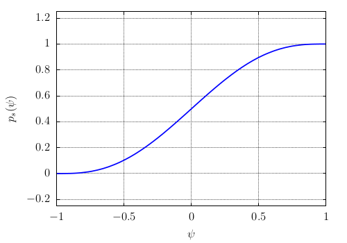
where \(p_{s}(\psi)\) is an interpolation polynomial defined by:

(519)\[p_{s}(\psi)=\frac{1+p(\psi)}{2}\]

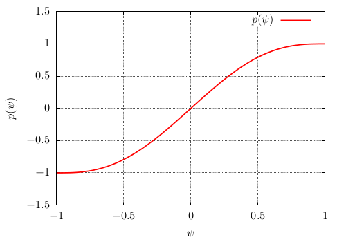
of minimum and maximum values between 0 and 1 (see Fig. Fig-Polynom-ps-psi). It is defined by \(p(\psi)\) of minimum and maximum values -1 and +1 (see Fig. Fig-Polynom-p-psi)

(520)\[p(\psi)=\frac{15}{8}\left[\psi-\frac{2}{3}\psi^{3}+\frac{\psi^{5}}{5}\right]\]

Fig. 55 Interpolation function \(p_s(\psi)\)

Fig. 56 Interpolation function \(p(\psi)\)

Variation of \(\mathscr{F}\)

The variation of \(\mathscr{F}\) writes:

(521)\[\delta\mathscr{F}=\int\left\{ -\zeta\boldsymbol{\nabla}^{2}\psi+f_{dw}^{\prime}(\psi)+\frac{p^{\prime}(\psi)}{2}\left[f_{s}(T)-f_{l}(T)\right]\right\} \delta\psi+\left\{ p_{s}(\psi)\frac{\partial f_{s}(T)}{\partial T}+[1-p_{s}(\psi)]\frac{\partial f_{l}(T)}{\partial T}\right\} \delta TdV\]

Temperature equation

Temperature equation

The conservation of internal energy density \(e\) writes:

(522)\[\frac{\partial e}{\partial t}=\boldsymbol{\nabla}\cdot(\Lambda\boldsymbol{\nabla}T)\]

where the Fourier law has been assumed for the diffusive flux. After expressing the internal energy \(e(\phi,s)\) as a function of \(T\) (see proof below), we obtain:

(523)\[\boxed{C_{p}\frac{\partial T}{\partial t}=\boldsymbol{\nabla}\cdot(\Lambda\boldsymbol{\nabla}T)-\underbrace{\frac{1}{2}p^{\prime}(\psi)\mathcal{L}\frac{\partial\psi}{\partial t}}_{\text{Latent heat at interface}}}\]

Proof

• Variation of \(\mathscr{F}\) wrt \(T\): opposite of entropy

  (524)\[\begin{split}s(\psi,T)&=-\frac{\delta\mathscr{F}}{\delta T}\\ &=-\frac{\partial f_{bulk}(\psi,T)}{\partial T}\\ &=-p_{s}(\psi)\underbrace{\frac{\partial f_{s}}{\partial T}}_{s_{s}(T)}-\left[1-p_{s}(\psi)\right]\underbrace{\frac{\partial f_{l}}{\partial T}}_{s_{l}(T)}\end{split}\]

• Thermo identity (\(de=Tds\)) and chain rule

  \[\begin{split}de&=Tds(\psi,T)\\ &=\underbrace{T\frac{\partial s}{\partial T}}_{C_{p}\text{: specific heat}}dT+T\underbrace{\frac{\partial s}{\partial\psi}}_{\text{use previous Eq.}}d\psi\end{split}\]

  For the first term of the right-hand side we use the definition of specific heat Eq. (). For the second term we derive Eq. () wrt \(\psi\). After division by \(dt\), we obtain

  (525)\[\frac{\partial e}{\partial t} =C_{p}\frac{\partial T}{\partial t}+p_{s}^{\prime}(\psi)\underbrace{T\left[s_{l}(T)-s_{s}(T)\right]}_{\equiv\mathcal{L}\text{: latent heat}}\frac{\partial\psi}{\partial t}\]

  Finally by replacing Eq. () in Eq. (), we obtain Eq. ().

Phase-field equation

The dynamic of \(\psi\) must obey to the following Allen-Cahn equation Eq. (451) to minimize the free energy:

(526)\[\frac{1}{\mathscr{M}_{\psi}}\frac{\partial\psi}{\partial t}=-\frac{\delta\mathscr{F}}{\delta\psi}\]

To calculate the variation of \(\mathscr{F}\) wrt \(\psi\), we use Eq. ():

\[\begin{split}\frac{1}{\mathscr{M}_{\psi}}\frac{\partial\psi}{\partial t}&={\color{gray}-\frac{\delta\mathscr{F}_{int}(\psi,\boldsymbol{\nabla}\psi)}{\delta\psi}}-\frac{\partial f_{bulk}(\psi,T)}{\partial\psi}\\ &={\color{gray}\zeta\boldsymbol{\nabla}^{2}\psi-f_{dw}^{\prime}(\psi)}-\underbrace{\frac{p^{\prime}(\psi)}{2}\left[f_{s}(T)-f_{l}(T)\right]}_{\text{Thermodynamic driving source}}\end{split}\]

To simplify the thermodynamic driving source, a common hypothesis is to consider the temperature \(T\) close to the melting temperature \(T_m\). A Taylor expansion yields:

(527)\[f_{\Phi}(T)\sim f_{\Phi}(T_{m})+\left.\frac{\partial f_{\Phi}}{\partial T}\right|_{T_{m}}(T-T_{m})\]

where \(\Phi=s,l\). At \(T_m\), \(f_l(T_m)=f_s(T_m)\) and the latent heat is () \(\mathcal{L}=T_{m}[s_{l}(T_{m})-s_{s}(T_{m})]\). Finally

\[\frac{1}{\mathscr{M}_{\psi}}\frac{\partial\psi}{\partial t}=\zeta\boldsymbol{\nabla}^{2}\psi-Hg_{3}^{\prime}(\psi)-\frac{p^{\prime}(\psi)}{2}\frac{\mathcal{L}}{T_{m}}(T-T_{m})\]

In the right-hand side, the coefficient \(H\) is set in factor:

(528)\[\frac{1}{\mathscr{M}_{𝜓}}\frac{\partial\psi}{\partial t}=H\left[\frac{\zeta}{H}\boldsymbol{\nabla}^{2}𝜓-g_{3}^{\prime}(𝜓)-\frac{1}{H}\frac{p^{\prime}(𝜓)}{2}\frac{\mathcal{L}}{T_{m}}(T-T_{m})\right]\]

and we define new coefficients:

Characteristic time

(529)\[\tau_{0}=\frac{1}{(H\mathscr{M}_{\psi})}\]

Interface width

(530)\[W_{0}=\sqrt{\frac{\zeta}{H}}\]

Coupling coefficient

(531)\[\lambda=\frac{1}{H}\]

Finally, using Eqs. (529), (530) and (531) in Eq. (528) we obtain for the phase-field equation:

Phase-field equation

(532)\[\tau_{0}\frac{\partial𝜓}{\partial t}=W_{0}^{2}\boldsymbol{\nabla}^{2}𝜓-g_{3}^{\prime}(𝜓)-\lambda\frac{p^{\prime}(𝜓)}{2}\frac{\mathcal{L}}{T_{m}}(T-T_{m})\]

Summary

Phase-field model of solidification

The phase-field model of solidification is composed of one phase-field equation for the interface:

(533)\[\tau_{0}\frac{\partial𝜓}{\partial t}=W_{0}^{2}\boldsymbol{\nabla}^{2}𝜓-g_{3}^{\prime}(𝜓)-\lambda\frac{p^{\prime}(𝜓)}{2}\frac{\mathcal{L}}{T_{m}}(T-T_{m})\]

coupled with one temperature equation:

(534)\[C_{p}\frac{\partial T}{\partial t}=\boldsymbol{\nabla}\cdot(\Lambda\boldsymbol{\nabla}T)-\underbrace{\frac{1}{2}p^{\prime}(\psi)\mathcal{L}\frac{\partial\psi}{\partial t}}_{\text{Latent heat at interface}}\]

Equivalence between phase-field model and Stefan’s problem

Equivalence between sharp and diffuse interface models

The sharp interface model (Stefan’s problem) and the phase-field model expressed with the dimensionless temperature \(\theta=(T-T_{m})C_{p}/\mathcal{L}\) write:

Stefan’s problem with dimnesionless temperature

\[\begin{split}\frac{\partial\theta}{\partial t}&=D\boldsymbol{\nabla}^{2}\theta\\ v_{n}&=D\hat{\boldsymbol{n}}\cdot(\boldsymbol{\nabla}\theta|_{sol}-\boldsymbol{\nabla}\theta|_{liq})\\ \theta_{i}&=-{\color{red}d_{0}}\kappa-{\color{red}\beta}v_{n}\end{split}\]

Phase-field model with dimensionless temperature

\[\begin{split}\frac{\partial\theta}{\partial t}&=D\boldsymbol{\nabla}^{2}\theta-\frac{1}{2}p^{\prime}(\psi)\frac{\partial\psi}{\partial t}\\ {\color{blue}\tau_{0}}\frac{\partial\psi}{\partial t}&={\color{blue}W_{0}^{2}}\boldsymbol{\nabla}^{2}\psi-g_{3}^{\prime}(\psi)-{\color{blue}\lambda}\frac{p^{\prime}(\psi)}{2}\theta\end{split}\]

where \(\theta\) is the dimensionless temperature, \(d_{0}=\sigma_{0}T_{m}C_{p}/\mathcal{L}^{2}\) is the capillary length, and \(\beta=C_{p}/\mathcal{L}m\) is the kinetic coefficient. With the matched asymptotic expansions, it is proved that both models are equivalent provided that the two following conditions hold:

(535)\[{\color{red}d_{0}}={\color{teal}a_{1}}\frac{{\color{blue}W_{0}}}{{\color{blue}\lambda}}\]

(536)\[{\color{red}\beta}={\color{teal}a_{1}}\left[\frac{{\color{blue}\tau_{0}}}{{\color{blue}\lambda}{\color{blue}W_{0}}}-{\color{teal}a_{2}}\frac{{\color{blue}W_{0}}}{D}\right]\]

where \({\color{teal}a_{1}}=0.8839\) and \({\color{teal}a_{2}}=0.6267\) (see [1]). In the right-hand side of Eqs. () and () \(\lambda\), \(W_{0}\) and \(\tau_{0}\) are the parameters of the phase-field model.

Anisotropy function and phase-field model of crystal growth

Dependence of properties with normal vector \(\boldsymbol{n}\equiv\boldsymbol{n}_{\psi}=-\boldsymbol{\nabla}\psi/\bigl|\boldsymbol{\nabla}\psi\bigr|\)

Surface tension \(\sigma\equiv\sigma(\boldsymbol{n})\)

(537)\[\sigma(\boldsymbol{n})=\sigma_{0}{\color{red}a_{s}(\boldsymbol{n})}\]

kinetic coefficient \(\beta\equiv\beta(\boldsymbol{n})\)

(538)\[\beta(\boldsymbol{n})=\beta_{0}{\color{red}a_{s}(\boldsymbol{n})}\]

Interface width \(W\equiv W(\boldsymbol{n})\)

(539)\[W(\boldsymbol{n})=W_{0}{\color{red}a_{s}(\boldsymbol{n})}\]

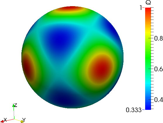
where the anisotropy function \(a_{s}(\boldsymbol{n})\) depends on the shape of crystal we want to simulate. The simplest one is the equiaxe crystal of main directions [100]

Definition of \(a_s(\boldsymbol{n})\)

(540)\[{\color{red}a_{s}(\boldsymbol{n})}=1+\epsilon_{s}\left[4(n_{x}^{4}+n_{y}^{4}+n_{z}^{4})-3\right]\]

where \(\epsilon\) is a positive parameter.

Fig. 57 Representation of anisotropy function \(a_s(\boldsymbol{n})\)

Phase-field model of crystal growth

Phase-field equation

(541)\[\tau_{0}{\color{red}a_{s}^{2}(\boldsymbol{n})}\frac{\partial\psi}{\partial t}=W_{0}^{2}\boldsymbol{\nabla}\cdot\left[{\color{red}a_{s}^{2}(\boldsymbol{n})}\boldsymbol{\nabla}\psi\right]+\boldsymbol{\nabla}\cdot{\color{blue}\boldsymbol{\mathcal{N}}(\boldsymbol{n})}+\underbrace{(1-\psi^{2})\left[\psi-\lambda\theta(1-\psi^{2})\right]}_{\text{source term of phase change (0 in bulks)}}\]

where

(542)\[{\color{blue}\boldsymbol{\mathcal{N}}(\boldsymbol{n})}=W_{0}^{2}\bigl|\boldsymbol{\nabla}\psi\bigr|^{2}{\color{red}a_{s}(\boldsymbol{n})}\frac{\partial{\color{red}a_{s}(\boldsymbol{n})}}{\partial(\partial_{\alpha}\psi)}\]

and the anisotropy function \(a_s(\boldsymbol{n})\) is defined by Eq. (540).

Temperature equation

The temperature equation remains unchanged:

(543)\[\frac{\partial\theta}{\partial t}=D\boldsymbol{\nabla}^{2}\theta+\frac{1}{2}\frac{\partial\psi}{\partial t}\]

References

[1]

Alain Karma and Wouter-Jan Rappel. Quantitative phase-field modeling of dendritic growth in two and three dimensions. Physical Review E, 57(4):pp. 4323–4349, 1998. doi:10.1103/PhysRevE.57.4323.

Section author: Alain Cartalade