Law of similarity: application on Poiseuille flow

To start practicing with input parameters without physical dimension, we recommmend to run the classical test case of Poiseuille flow which is contained in folder run_training_lbm. The law of similarity is applied to derive dimensionless parameters from physical parameters in SI units. In the case of Poiseuille flow, Reynolds number is used to derive dimensionless parameters.

The analytical solution of Poiseuille flow is

(18)\[u_{x}(y)=u_{max}\left(1-\frac{4y^{2}}{L^{2}}\right)\]

where \(u_{max}=gL^{2}/8\nu\). If we consider water properties inside a channel of width \(L\)

Parameter	Math symbol	Value	Dimension
Gravity	\(g\)	\(9.81\cong10\)	m/s2
Density	\(\rho_w\)	\(998.29\cong1000\)	kg/m3
Kinematic viscosity	\(\nu\)	\(10^{-6}\)	m2/s
Width	\(L\)	\(10^{-3}\)	m

it is possible to compute the maximum velocity \(u_{max}\)

(19)\[u_{max}=\frac{gL^{2}}{8\nu}=1.25\text{ m.s}^{-1}\]

and the Reynolds number Re:

(20)\[\text{Re}=\frac{u_{max}L}{\nu}=1250\]

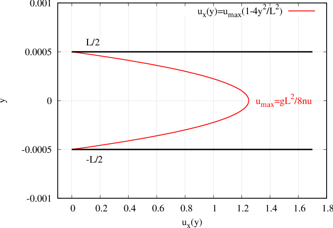
Fig. 30 Poiseuille flow inside a channel

In what follows, we present four different ways to set one characteristic length and one characteristic time to derive all dimensionless parameters.

First choice of parameters: \(\delta x_1\) and \(\tau\)

If we set (initial guess) \(\delta x_1=5 \times 10^{-5}\) m and \(\tau=0.6\), then we derive the other parameters

\[L_{1}^{\star}=\frac{L}{\delta x_{1}}=20\]

where \(L_1^{\star}\) is the dimensionless width of domain, obtained from the space-step \(\delta x_1\). It is equivalent to the total number of nodes \(N_y\).

The kinematic viscosity is linked to the collision rate:

\[\nu_{1}^{\star}=\frac{1}{3}(\tau-0.5)=0.03333\]

We can derive the time step:

\[\delta t=\frac{1}{3}(\tau-0.5)\frac{\delta x_{1}^{2}}{\nu}=8.33\times10^{-5}\]

Unstable simulation

For a given Re number \(\text{Re}=u_{max}^{\star}L^{\star}/\nu^{\star}=1250\), the maximum dimensionless velocity is:

\[u_{max}^{\star}=\frac{\nu^{\star}\text{Re}}{L^{\star}}=2.08\]

That value is greater than \(\color{red}{u_{max}^{\star}}{\color{red}{\gg0.4}}\) so that the simulation will be unstable.

Second choice of parameters: \(L^{\star}\) and \(\nu^{\star}\)

From the previous set of parameters, one solution to keep the simulation stable is to set \(L^{\star}\) and \(\nu^{\star}\) such that \(u_{max}^{\star}/10=0.208\). To achieve that, for a given Reynolds number, it is sufficient to multiply by five the dimensionless width \(L_{1}^{\star}\times5\) and divide by two the kinematic viscosity \(\nu_{1}^{\star}/2\).

• \(L^{\star}=L_{1}^{\star}\times5=100\), means that the number of nodes is \(N_y=100\). We can derive the space-step by:

  (21)\[\delta x=\frac{L}{L^{\star}}=10^{-5}\]

• The target value of dimensionless kinematic viscosity is

  (22)\[\nu^{\star}=\frac{\nu_1^{\star}}{2}=0.016667\]

We can derive the collision rate which is linked to kinematic viscosity by \(\tau^{\star}=3\nu^{\star}+0.5=0.55\).

• We can derive the time step, for example here with the kinematic viscosity:

  (23)\[\delta t=\frac{1}{3}(\tau-0.5)\frac{\delta x^{2}}{\nu}=1.6667\times10^{-6}\]

• Finally, the dimensionless gravity \(g^{\star}\) is obtained from the physical value of gravity and the factor of conversion \(C_g=\delta x/\delta t^2\) (see Eq. (15)):

  (24)\[g^{\star}=g\frac{\delta t^{2}}{\delta x}=2.777\times10^{-6}\]

The simulation is accurate because \(u_{max}^{\star}<0.3\) and stable because \(u_{max}^{\star}<0.4\).

Parameters of input file

For test case TestCase02_Poiseuille_Water of folder run_training_lbm, those values are set in the .ini input file. The main parameters are presented below:

[run]
dt=1

[mesh]
ny=100
ymin=-50
ymax=50

[params]
rho0=1
rho1=1
nu0=0.01666666666666668
nu1=0.01666666666666668
gx=2.777777777777784e-06

• dt=1 means that \(\delta t^{\star}=1\)

• The number of nodes \(N_y\) in \(y\)-direction is ny=100

• The width of domain (\(L^{\star}\)) is ymax-ymin=100 meaning that \(\delta x^{\star}=L^{\star}/N_y=1\)

• The value of kinematic viscosities nu0 and nu1 are given by Eq. (22)

• The dimensionless gravity is given by Eq. (24)

  Once the simulation is complete, use \(\delta x\) defined by Eq. (21), \(\delta t\) defined by
  Eq. (23), and the density to calculate the conversion factors Eqs. (15).
  Use those conversion factors to obtain the results with physical dimensions.
  A python script Post-Pro_Poiseuille_Water_CompareAnaly.py is available
  in the folder to compare numerical and analytical solutions.

For LBM training session

Those stages are written in a python script:

$ cd TestCase02_Poiseuille_Water
$ python Pre-Pro_Poiseuille.py

For training session

$ gedit TestCase02_Poiseuille_Water&

Check that the numerical parameters of your input file correspond to the output of python script.

The methodology is described in the jupyter notebook Validation-Sheet_Poiseuille_Similarity_Water.ipynb. The input parameters of TestCase02_Poiseuille_Water.ini are dimensionless.

$ cd run_training_lbm/TestCase02_Poiseuille_Water
$ jupyter notebook Validation-Sheet_Poiseuille_Similarity_Water.ipynb

Third choice of parameters: \(u_{max}^{\star}\) and \(\tau\)

As unit of length and time, it is also possible to set \(u_{max}^{\star}=0.1<0.4\) and \(\tau=0.8>052\). The simulation will be stable and accurate. In order to derive the other parameters, we use the first one to calculate de conversion factor of velocity:

\[C_{u}=\frac{u_{max}}{u_{max}^{\star}}=12.5=\frac{\delta x}{\delta t}\]

Newt we use the relaxation rate for deriving the dimensionless kinematic viscosity:

\[\nu^{\star}=\frac{1}{3}(\tau-0.5)=0.1\]

and the conversion factor of \(\nu\):

\[C_{\nu}=\frac{\nu}{\nu^{\star}}=10^{-5}=\frac{\delta x^{2}}{\delta t}\]

The dimensionless width (or number of nodes) is derived from the Reynolds number

\[L^{\star}=\frac{\text{Re}\nu^{\star}}{u_{max}^{\star}}=1250\]

Remark

That set of initial parameters requires a discretization with 1250 nodes. The simulation won’t be efficient.

The ratio between both conversion factors allows deriving the space-step

\[\delta x=\frac{C_{\nu}}{C_{u}}=8\times10^{-7}\quad{\color{gray}(\text{check }=L/L^{\star})}\]

Finally, \(\delta t\) can be obtained

\[\delta t=\frac{\delta x}{C_{u}}=6.4\times10^{-8}\quad{\color{gray}(\text{check }\nu=\nu^{\star}\delta x^{2}/\delta t)}\]

as well as \(g^{\star}\):

\[g^{\star}=g\frac{\delta t^{2}}{\delta x}=5.12\times10^{-8}\]

Fourth choice of parameters: \(u_{max}^{\star}\) and \(L^{\star}\)

Another choice of parameters is possible. Set for instance \(L^{\star}=5\times 10^{2}\) and \(u_{max}^{\star}=0.1<0.4\). In that case, we can derive the missing parameters as follows:

\[\delta x=\frac{L}{L^{\star}}=2\times10^{-6}\]

\[C_{u}=\frac{u_{max}}{u_{max}^{\star}}=12.5=\frac{\delta x}{\delta t}\]

\[\delta t=\frac{\delta x}{C_{u}}=1.6\times10^{-7}\]

\[\nu^{\star}=\frac{u_{max}^{\star}L^{\star}}{\text{Re}}=0.04\quad{\color{gray}(\text{check }\nu=\nu^{\star}\delta x^{2}/\delta t)}\]

\[\tau=3\nu^{\star}+0.5=0.62\;({\color{red}>0.55})\]

\[g^{\star}=g\frac{\delta t^{2}}{\delta x}=1.28\times10^{-7}\]

Conclusion

Conclusion

On that simple Poiseuille flow, we see that several ways are possible to set two initial parameters and derive all others. For other configurations and types of flows, those choices depend on the system and phenomenology to be simulated. The example was given here for a single-phase flow. For two-phase flows, one example is detailed in Law of similarity: practice on Rayleigh-Taylor instability. To help users to set dimensionless parameters, several python scripts are available in the test cases of run_training_lbm. A description of one of them is done in Law of similarity: practice on Rayleigh-Taylor instability.