Binary dissolution

Compilation of kernel GPMixt

Compilation on A6000

Makefile for GPU of manwe server

• For cuda on GPU A6000 of manwe Go to folder LBM_Saclay_Rech-Dev

$ cd LBM_Saclay_Rech-Dev

and execute the configure_build.sh script to create the makefile

$ ./compilation/manwe/cuda_a6000/configure_build.sh

will return:

The following problems are currently implemented:
0  AC
1  Advection-Diffusion
2  Crystal_growth_Younsi
3  GPMixt
4  GPMixtNS
5  GPMixtTernary
6  GPMuTernary
7  MPwSLphC
8  NS
9  NS_3phases_1comp_phase_change
10 NSAC_Comp
11 NSAC_Comp_3phases
12 NSAC_Comp_3phases3D
13 NSAC_coupling
14 NSAC_Fakhari
15 NSAC_Surfactant
Choose which problems to include by indicating a list of space or comma separated numbers, eg '0 1' or '0,1'.
Write 'all' to include all problems.
Problem numbers:

Compilation

Write 3 for GPMixt kernel

Problem numbers: 3

Go to the directory that is indicated by the green link, e.g., if number 3 has been set for GPU:

$ cd LBM_Saclay_Rech-Dev/build_cuda_a6000/build_GPMixt

Compile:

$ make -j 22

Run test cases

Stefan problem with \(D_s \sim D_l\)

Run Stefan problem

1. Go to the folder of Stefan problem

$ cd run_training_dissolution/01_Binary_Stefan-Problem

2. Run the test case on volatile of manwe

$ LBM_Saclay_Rech-Dev/build_cuda_a6000/build_GPMixt/src/LBM_saclay d2q9_1d_Stefan.ini

3. Post-process with paraview12

$ paraview12&

Commands in paraview12

For interface positions

1. Open all vti files LBM_D2Q9_Stefan_

2. Ctrl space and Cell Data to Point Data and Apply

3. Clic on contour and select field phi with value 0.5 and Apply

4. File –> Save Data, choose .cvs format. Select it and write the file name: interface

5. Clic on Write Time Steps and Write Time Steps Separately and OK

For composition profile

1. Open file LBM_D2Q9_Stefan_FINAL.vti

2. Ctrl space and Cell Data to Point Data and Apply

3. Ctrl space + Plot Over Line

4. Select Sample At Segment Centers Clic on X axis and Apply –> new graph with profile

5. File –> Save Data, file name: profil_comp_100.csv and OK

Next in your terminal

Run python script

$ python Post-Pro_Compare_Analytical-Solution.py

You must obtain Fig. 30

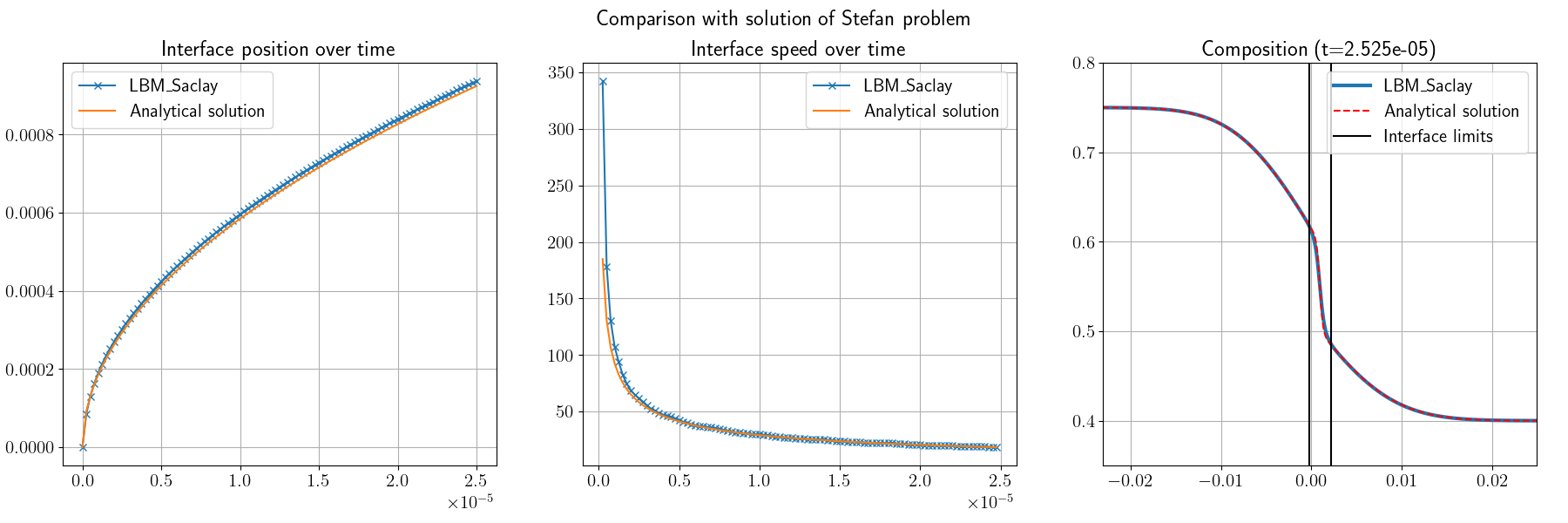
Fig. 30 Comparison between analytical solution of Stefan problem and LBM_Saclay with GPMixt kernel

Stefan problem with \(D_s=0\)

1. Without anti-trapping current

Run first test case without anti-trapping current

1. Go to the folder of Stefan problem

$ cd /run_training_dissolution/02_Binary_Anti-Trapping-Current

2. Run the first test case without anti-trapping current

$ LBM_Saclay_Rech-Dev/build_cuda_a6000/build_GPMixt/src/LBM_saclay Test_1d_Stefan_Ds0_no-anti-trapping.ini

3. Post-process with paraview12

$ paraview12&

Commands in paraview12

For interface positions

1. Open all vti files LBM_Stefan_Ds0_no-anti-trapping

2. Ctrl space and Cell Data to Point Data and Apply

3. Clic on contour and select field phi with value 0.5 and Apply

4. File –> Save Data, choose .cvs format. Select it and write the file name: interface

5. Clic on Write Time Steps + Write Time Steps Separately + Choose Arrays To Write + unslect phi + OK

For composition profile

1. Open file LBM_Stefan_Ds0_no-anti-trapping_FINAL.vti

2. Ctrl space and Cell Data to Point Data and Apply

3. Ctrl space + Plot Over Line

4. Select Sample At Segment Centers Clic on X axis and Apply –> new graph with profile

5. File –> Save Data, file name: profil_comp.csv and OK

Next in your terminal

For training session: python script

$ python Script_plot-Stefan1D_anti-trapping.py

You must obtain Fig. 31

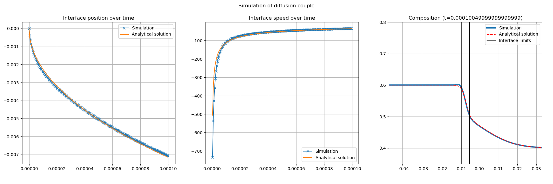
Fig. 31 Comparison between analytical solution of Stefan problem with \(D_s=0\) and LBM_Saclay without anti-trapping current

2. With anti-trapping current

Exercise

Start again with LBM_Saclay input file Test_1d_Stefan_Ds0_with-anti-trapping.ini and compare the composition profile. You must obtain Fig. 32

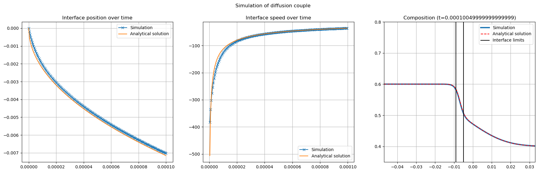
Fig. 32 Comparison between analytical solution of Stefan problem with \(D_s=0\) and LBM_Saclay with anti-trapping current

Simulation of porous medium dissolution

Porous medium geometry

Description of porous medium geometry

The porous medium geometry is described in the datafile image_niv1_slice0.dat.

This is a text file with format

i,j,k,value

where i, j, k are the positions of x, y, z and value is 0 or 1. The file contains 256x256x237 values.

i.e. for the first ten lines:

0,0,0,1
1,0,0,1
2,0,0,0
3,0,0,0
4,0,0,0
5,0,0,0
6,0,0,0
7,0,0,0
8,0,0,0
9,0,0,0
...

Options in LBM_Saclay input file

The datafile name of porous geometry must be set in the input file of LBM_Saclay in the [init] section with init_type=data

[init]
init_type=data
data_file=./image_niv1_slice0.dat
sizeRatio=2
initCl=0.4
initCs=0.6

The file image_niv1_slice0.dat is used to initialize the phase-field \(\phi(\boldsymbol{x},0)\). Next, the composition is initialized with \(\phi(\boldsymbol{x},0)\) and \(c_l^0\) (initCl) and \(c_s^0\) (initCs).

The mesh of the that test case is composed of nx=512 and ny=512 cells (see section [mesh]). The datafile image_niv1_slice0.dat contains only 256 values for i and 256 values for j. The input file is rescaled with the option sizeRatio=2. For using the same datafile on a mesh composed of 1024x1024 cells, the option must be set to sizeRatio=4.

Run simulation of porous medium dissolution

Go to folder 03_Binary_Porous-Medium and run LBM_Saclay with the .ini input file:

$ cd run_training_dissolution/03_Binary_Porous-Medium
$ LBM_Saclay_Rech-Dev/build_cuda_a6000/build_GPMixt/src/LBM_saclay Test_Dissolution_Porous-Medium.ini

Post-process with paraview12

Commands in paraview12

1. Open all vti files Test_Dissolution_Porous-Medium

2. Load paraview state State-Paraview_5-12_Porous-Medium.pvsm

At initial time of simulation you must obtain Fig. 33. At final time of simulation, you must obtain Fig. 34.

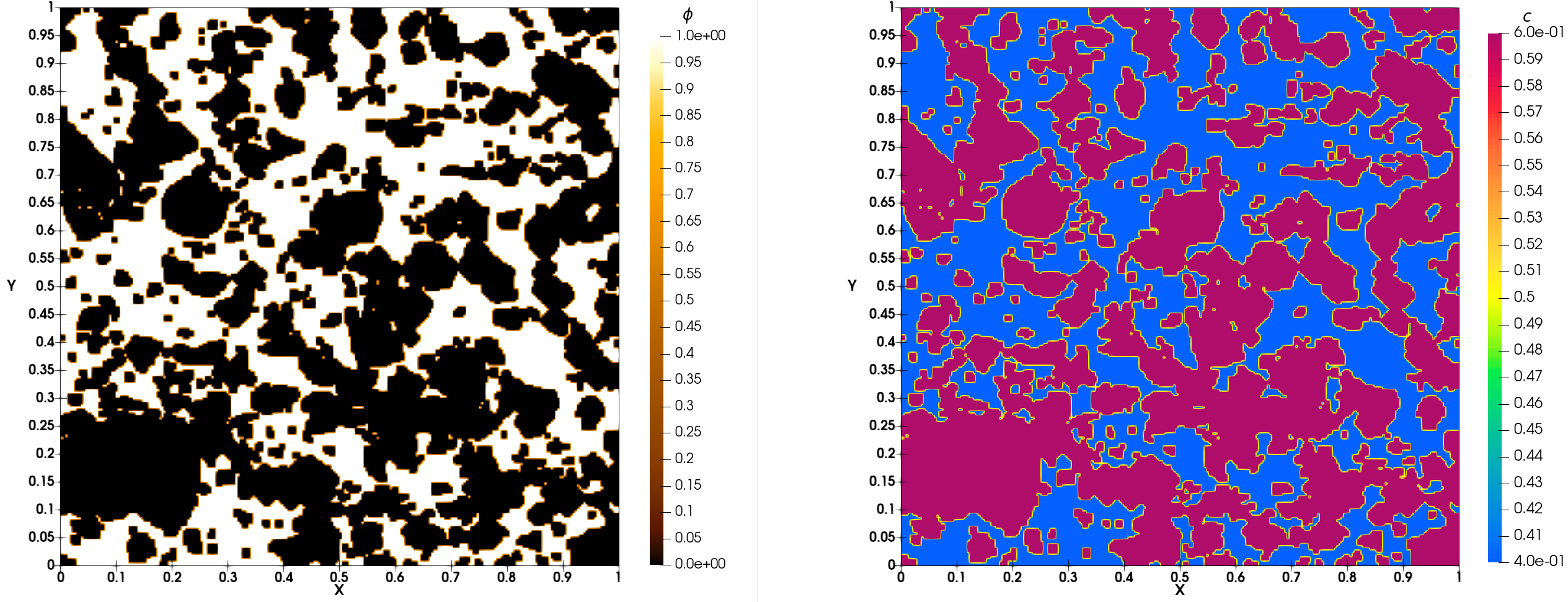
Fig. 33 Simulation of porous medium dissolution: initial time

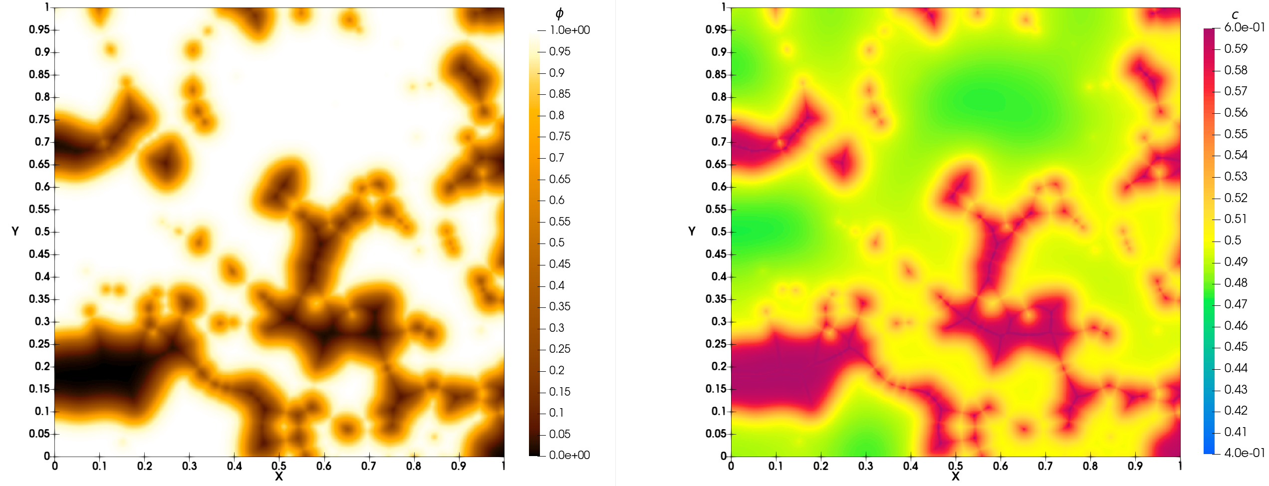
Fig. 34 Simulation of porous medium dissolution: final time